

The Calm Before More Calm: the TTM Squeeze, the Bollinger Squeeze and volatility clustering in twenty years of S&P 500 stocks
Chart books call the squeeze the calm before the storm: when a stock's Bollinger Bands slip inside its Keltner Channel, a big move is supposed to be near. Econometricians say calm is followed by more calm, and volatility by more volatility. We measured both on S&P 500 stocks from 2006 to 2025, against every trading day of every member with prices on file. Volatility clustering held. The calmest days were followed by the calmest weeks and the most volatile days by the most volatile weeks. The squeeze added little of its own. The week after its signal was calmer than an ordinary week when it gave an upward signal and more volatile when it gave a downward signal, and most of that came from the direction of the price, about as after any rising or falling day. The reason is in how the squeeze is built. It measures a price going sideways, and a sideways price can be calm or volatile. Buying the upward breakout as the books teach it lost money over the twenty years, and so did a plain breakout over the previous month, while holding SPY multiplied $1 about fivefold.
Why this one
The squeeze is one of the most quoted setups in trading. John Bollinger wrote that when his bands narrow, a sharp move tends to follow. John Carter's TTM Squeeze put the idea on millions of charts: the dots stay red while the Bollinger Bands sit inside the Keltner Channel, and the trade is taken on the day they come out. Traders have a name for it: the calm before the storm.
Economists have another name for the same calm. Benoit Mandelbrot noticed in 1963 that large price changes tend to follow large ones and small changes small ones. Robert Engle and Tim Bollerslev built that into ARCH and GARCH, the models risk desks use every day. On their reading a squeeze does not announce a big move. It announces more calm.
Both readings take a squeeze to be a calm stock, so both are about the same days, and they cannot both be right. This study counts what came next every time a squeeze gave a signal in an S&P 500 stock over twenty years, and checks how calm those stocks were in the first place.
What we tested
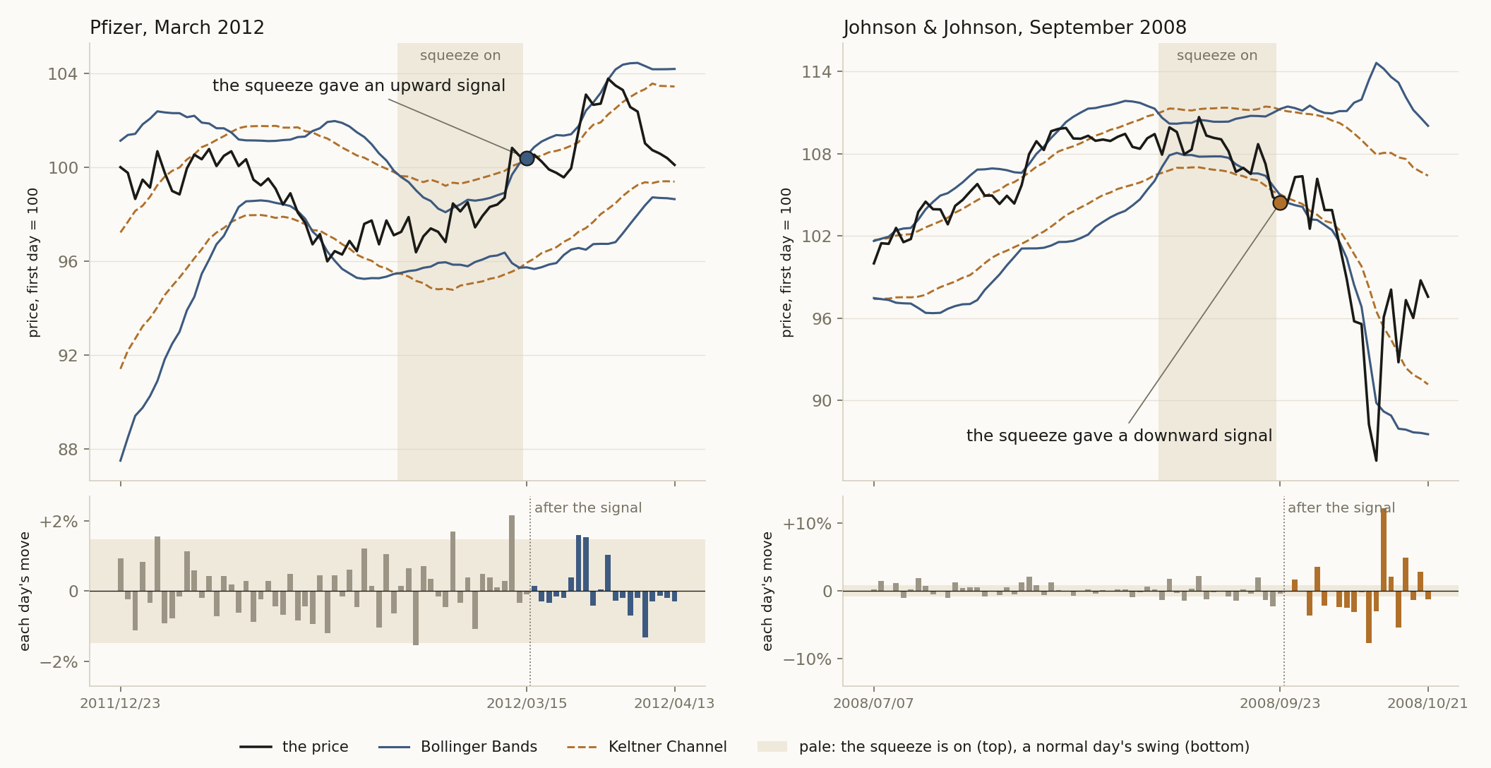
Figure 1 shows the setup on two real stocks. Bollinger Bands sit two standard deviations above and below the 20-day average of the price, so they widen when the price wanders and narrow when it settles. The Keltner Channel sits one and a half times the average daily range above and below the same average. When the bands slip inside the channel, the squeeze is on. It gives its signal on the first day they come back out, upward when Carter's momentum line is above zero and downward when it is below.
We asked four questions: does calm follow calm, does a big move follow a squeeze, does the direction of the break matter, and does the answer hold across settings and sectors.
The yardstick is an ordinary week. We took every trading day of every member of the index with prices on file, over the same twenty years, and measured the week after it the same way as the week after a squeeze: how much the stock swung from day to day, against the swing of its own past year. A squeeze has to look different from that to mean anything.
We ran 36 versions of the squeeze, and Carter's own setting inside each of eleven sectors, so the answer does not rest on one setting. Four of the 36 gave too few signals to count.
1 Methodology, in detail (click to open)
1 Methodology
Universe and window. Every member of the S&P 500 as the index stood at the start of each year, 2006 to 2025, in twenty one-year windows, each registered and run in turn; nothing was changed between windows. Prices are daily closes without dividends.
The squeeze, as the platform runs it. The TTM Squeeze is on when the Bollinger Bands (the 20-day simple average of the close plus and minus two standard deviations) sit inside the Keltner Channel (the same simple average plus and minus a multiple of the simple average of the true range, over the same length). Because both share one midline, only the ratio of the two widths decides it, so the bands were held at two deviations and the channel moved: 1.0, 1.5 (Carter's classic) and 2.0 times the range. Lengths were 10, 20 and 30 days, the true range averaged over the same length, and the squeeze had to be on for at least 1, 5 or 20 days: 27 settings. It gives its signal on the first day the bands come back out, upward when Carter's momentum line is above zero and downward when it is below. Bollinger's own squeeze is on when the band width is at its lowest of the last 60, 125 or 250 sessions and gives its signal on the first close outside the bands, upward above the upper band and downward below the lower one, at lengths of 10, 20 and 30: 9 settings. Carter's setting (length 20, channel 1.5, at least 5 days inside) is the one used for Figures 1 to 4, the sectors and the trade. 32 of the 36 settings had at least 15 years with 20 or more signals in both directions; only those are drawn and counted.
What was measured. For every signal, from the close of the signal day, over the next 5, 20 and 60 sessions: the day-to-day swing (the standard deviation of daily log returns) against the stock's own over the 252 sessions up to the signal day, and the size of the move against the stock's median move over as many sessions within those same 252. Nothing after the signal day enters either yardstick. Each year's signals give one median; a year counts with at least 20 signals.
An ordinary week. The same arithmetic on every trading day of every member the index had at the start of each year gives each year's ordinary week. Figures 2, 4 and 5 and both tables divide by it, so 100 is what any week did; the swing of five days runs low against a year's on any week, and the division cancels that. Figure 3 counts weeks against the stock's own past year and shows any week beside the squeezes. The ten groups of Figure 2 sort each day by its swing over the last 20 sessions against the past year's, as the platform does to pick days as calm as a signal day; the rising and falling days split every day by the sign of Carter's momentum line, squeeze or not. Recomputed this way, every year's median after a signal matches the registered study's.
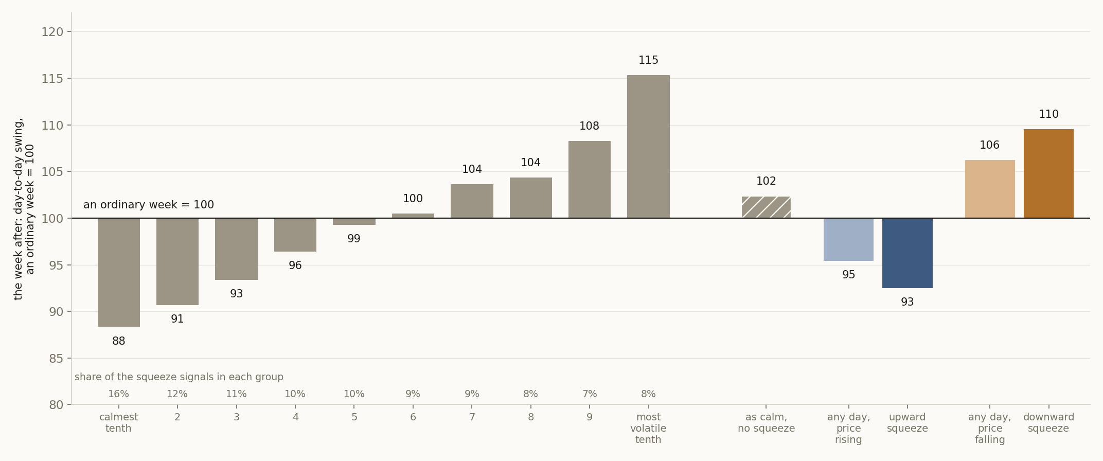
The days as calm as the signal days. For each signal the platform draws up to three days of the same stock, in the same tenth as the signal day and at least 20 sessions from any signal. That last condition keeps days near a squeeze out, and the days left came out more volatile than the ten groups alone would predict for the signal days (102 against about 98), probably because of it. The paper therefore also sets the squeezes against any rising and falling day.
The trades. Carter's setting was traded long only, ten stocks at most, equal weight, first come first served, 0.1% on every trade: buy on an upward signal, sell on a close below the 20-day average. A plain breakout (a close above the highest high of the previous 20 sessions, the same exit) was its comparison. Over the twenty years the squeeze breakout turned $1 into $0.37, the plain breakout into $0.70, and SPY's price alone into $5.04. Each family of settings traded its own middle setting the same way. None beat SPY.
Registration. The main study and five further studies (lengths 10, 20 and 30, Bollinger's own, and the sectors) were registered and run as separate studies, twenty windows each: 116 measurements in all. H1 to H3 were written in the design note at 19:24 UTC on 10 October 2026, before the first window was registered at 21:53 UTC; H4 is in the registration record.
What we wrote down before the first window was run, and what came back: - H1, the chart lore: twenty sessions after a signal, moves are larger than the stock's normal. After an upward signal, no. After a downward signal, slightly: about 7% larger than an ordinary month's move. - H2, clustering: five sessions after a signal the swing is below normal, and back to normal by sixty. Against the stock's past year it was below in every year, but so was an ordinary week. Against an ordinary week, the week after an upward signal was calmer and the week after a downward signal more volatile, and by sixty sessions both were within a few points of an ordinary stretch. - H3, the pinch itself: a squeeze is followed by a bigger swing than days just as calm without one. After a downward signal, yes. After an upward signal, the opposite. Those calm days came out at about an ordinary week (102). - H4, the trade: the squeeze breakout beats the plain breakout. It did not, and neither beat holding SPY.
2 Results
Findings
Does calm follow calm? Yes. Sort every day of every stock into ten groups by how much it had swung over its last four weeks, against its own past year (Figure 2). The calmest tenth of days was followed by a week about 12% calmer than an ordinary week, the most volatile tenth by a week about 15% more volatile, and the calm end came out calmer in every one of the twenty years. That is volatility clustering.
Does a big move follow a squeeze? Not much. After an upward squeeze the next week was about 7% calmer than an ordinary week, and after a downward squeeze about 10% more volatile, mostly because the price was falling; each held in 18 of the 20 years (Figure 4). Figure 3 shows the same split as odds. The split was wider in the first ten years than in the last ten. Since 2016 the week after an upward squeeze has been close to an ordinary week, and in 2024 it was more volatile than the week after a downward one.
Does the direction matter? Yes, but mostly as the direction of the price. On any day when Carter's momentum line pointed down, squeeze or no squeeze, the next week was about 6% more volatile than an ordinary week, and on any day it pointed up about 5% calmer. The squeeze added a point or two on the upward side and nothing measurable on the downward side. The upward squeeze came out calmer than an ordinary rising day in 13 of the 20 years, with one more tied, and the downward squeeze more volatile than an ordinary falling day in only 11. Days as calm as the signal days, with no squeeze, came out at about an ordinary week (Figure 2).
Does it hold everywhere? At every setting that gave signals often enough to count, the week after an upward squeeze was calmer than an ordinary week and calmer than the week after a downward one (Figures 5 and 6). The downward side was more volatile than ordinary at most settings and a little calmer than ordinary at a few of Bollinger's own settings and the tightest channel's longer lengths. In every sector the upward week was calmer than the downward one, widest apart in energy and technology and closest in health care.
2.1 Headline
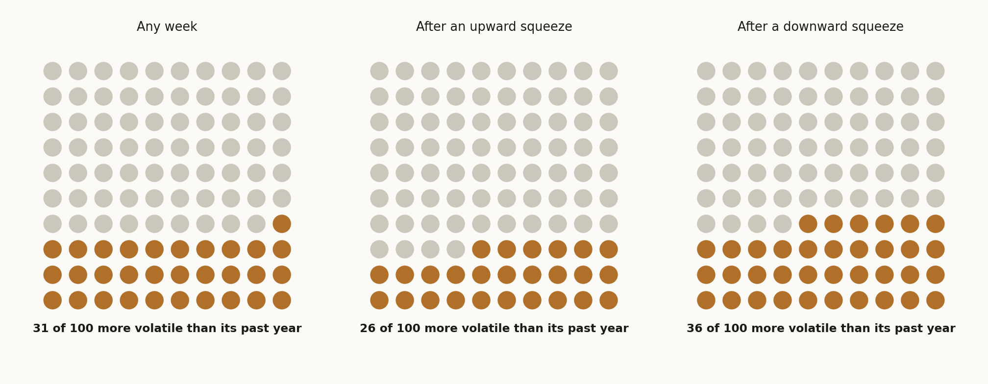
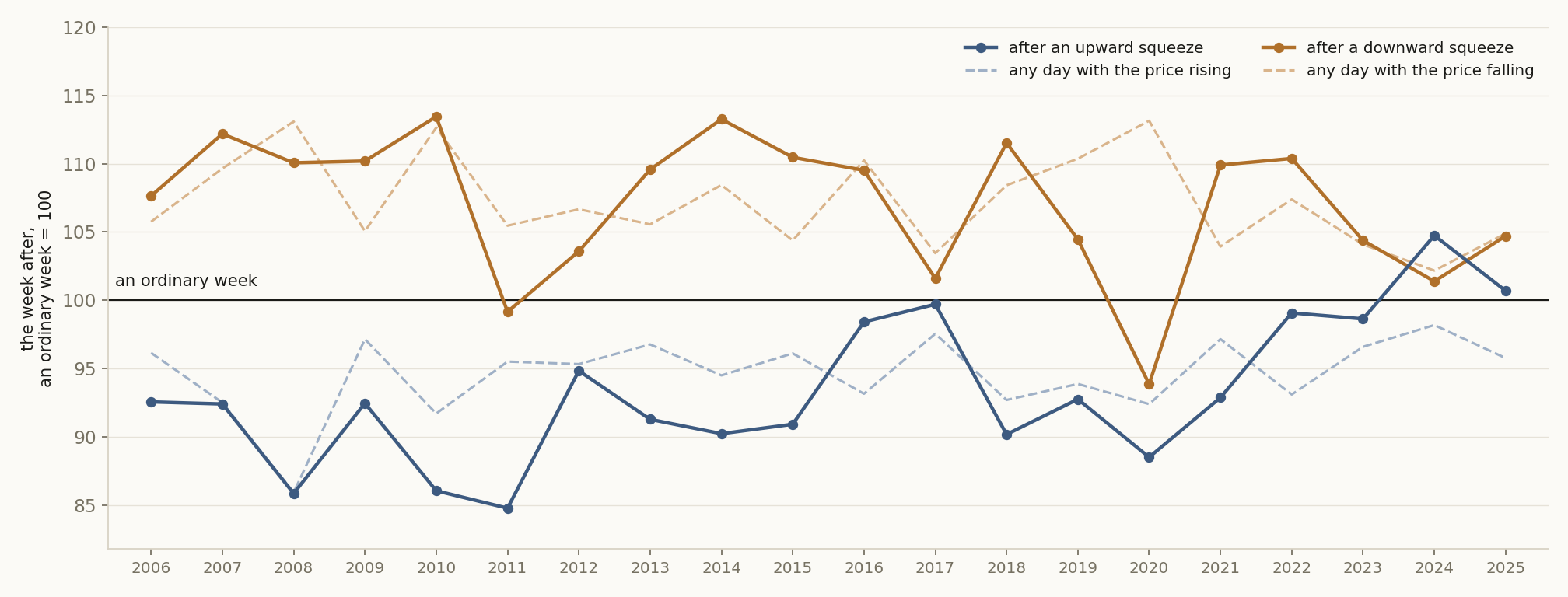
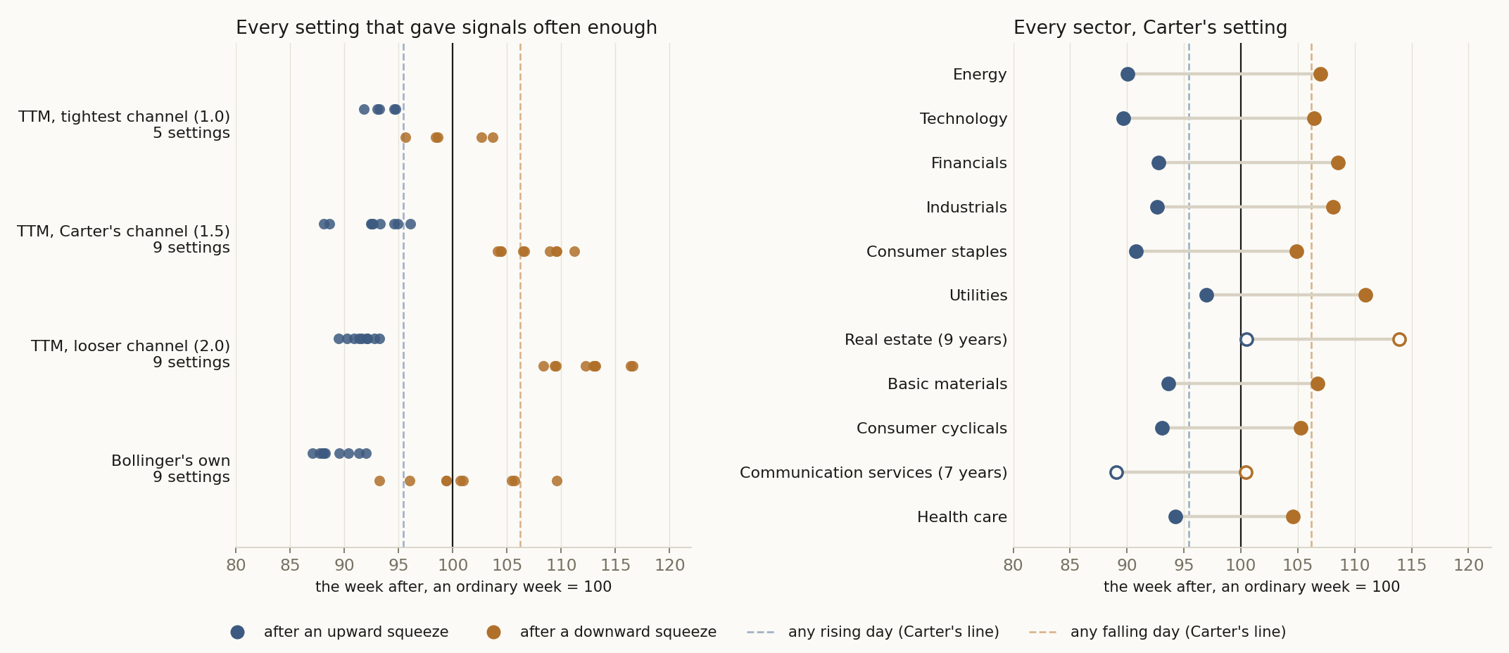
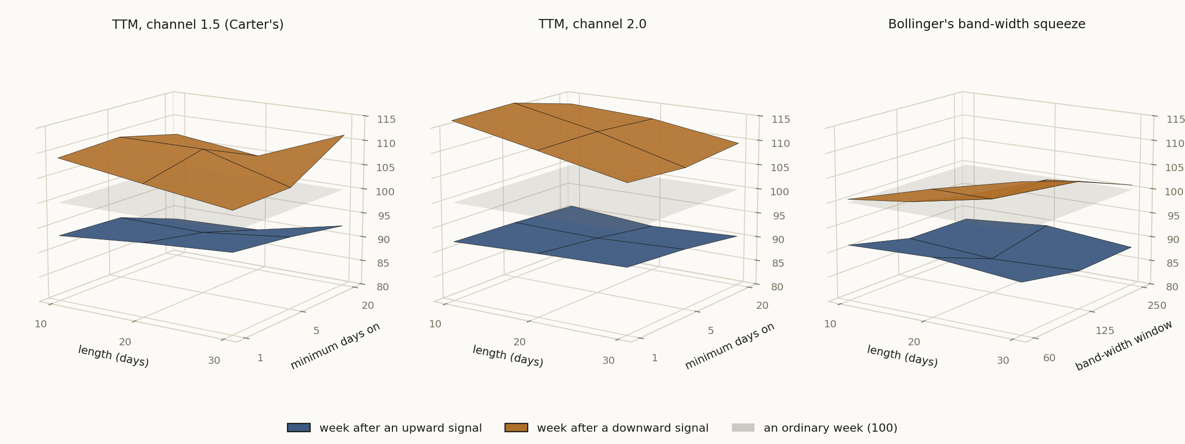
Table 1. The typical stock's day-to-day swing in the week after a signal, with each year's ordinary week at 100 (every day of every member with prices on file) and the median over the years, the range across each family's settings. Settings that gave too few signals to count are left out.
| The squeeze | Settings counted | After an upward squeeze | After a downward squeeze |
|---|---|---|---|
| TTM, tightest channel (1.0) | 5 | 92 to 95 | 96 to 104 |
| TTM, Carter's channel (1.5) | 9 | 88 to 96 | 104 to 111 |
| TTM, looser channel (2.0) | 9 | 89 to 93 | 108 to 117 |
| Bollinger's own | 9 | 87 to 92 | 93 to 110 |
Table 2. The same inside each sector, against the whole market's ordinary week (100), widest gap between the two directions first; gaps from unrounded values. Real estate and communication services have few years.
| Sector | Years | After an upward squeeze | After a downward squeeze | Gap |
|---|---|---|---|---|
| Energy | 20 | 90 | 107 | 17 |
| Technology | 20 | 90 | 106 | 17 |
| Financials | 20 | 93 | 109 | 16 |
| Industrials | 20 | 93 | 108 | 15 |
| Consumer staples | 20 | 91 | 105 | 14 |
| Utilities | 20 | 97 | 111 | 14 |
| Real estate | 9 | 101 | 114 | 13 |
| Basic materials | 20 | 94 | 107 | 13 |
| Consumer cyclicals | 20 | 93 | 105 | 12 |
| Communication services | 7 | 89 | 100 | 11 |
| Health care | 20 | 94 | 105 | 10 |
Sections 2.2 to 3, the full record: every year, every test, and how each one was run (click to open)
The registration names the two groups compared Squeeze breakout and Plain breakout; this paper calls them The squeeze breakout and The plain breakout.
2.2 Per-step results
| # | Out-of-sample window | The squeeze breakout SR | The plain breakout SR |
|---|---|---|---|
| 1 | 2006-01-03 → 2006-12-29 | 0.56 | -0.45 |
| 2 | 2007-01-03 → 2007-12-31 | -0.75 | -0.73 |
| 3 | 2008-01-02 → 2008-12-31 | -2.31 | -1.85 |
| 4 | 2009-01-02 → 2009-12-31 | -0.16 | 0.41 |
| 5 | 2010-01-04 → 2010-12-31 | -0.32 | 0.14 |
| 6 | 2011-01-03 → 2011-12-30 | -1.57 | -0.54 |
| 7 | 2012-01-03 → 2012-12-31 | 0.98 | 0.43 |
| 8 | 2013-01-02 → 2013-12-31 | 1.33 | 1.41 |
| 9 | 2014-01-02 → 2014-12-31 | -0.26 | 0.60 |
| 10 | 2015-01-02 → 2015-12-31 | -0.28 | -0.41 |
| 11 | 2016-01-04 → 2016-12-30 | 0.22 | 0.32 |
| 12 | 2017-01-03 → 2017-12-29 | 1.35 | 1.18 |
| 13 | 2018-01-02 → 2018-12-31 | -2.05 | -1.07 |
| 14 | 2019-01-02 → 2019-12-31 | 0.71 | 1.66 |
| 15 | 2020-01-02 → 2020-12-31 | 0.34 | -0.04 |
| 16 | 2021-01-04 → 2021-12-31 | 1.21 | 1.94 |
| 17 | 2022-01-03 → 2022-12-30 | -0.97 | -0.90 |
| 18 | 2023-01-03 → 2023-12-29 | 0.73 | 1.19 |
| 19 | 2024-01-02 → 2024-12-31 | -0.12 | 0.48 |
| 20 | 2025-01-02 → 2025-12-31 | -1.23 | -0.95 |
2.3 Search accounting
No search record exists for this design. It was not promoted from a recorded evolving search, so the number of alternatives tried before it, on paper, in another tool, or in the author's head, is unknown. Unknown is a different fact from one: a study with no lineage is not a strategy with one trial, it is a strategy with an unrecorded number of them. Accordingly no count of alternatives tried is claimed, and nothing in this paper is corrected for a search that was never recorded; the number that stands is the raw out-of-sample result plus this disclosure. The registered per-step record below (§4) still guarantees each window's hypothesis was hashed and registered before that window was scored.
2.4 The comparison
Both arms trade the same registered windows, so their returns can be PAIRED: inside each window the two return series are inner-joined date by date and the difference rThe squeeze breakout − rThe plain breakout is the object under test. Because this is ONE pre-declared contrast, frozen at registration before any window was scored, the paired statistic needs no multiple-testing deflation, and the per-arm pooled numbers above are likewise uncorrected, because this design has no recorded search to correct against (§2.3). The paired contrast carries that gap differently from the arm levels: it was declared before each window ran and it is scored on the difference, so no window could be read first and scored after. What the timestamps cannot speak to is how this contrast came to be the declared one, which is the limit §2.3 states.
In the table: Arm A = The squeeze breakout · Arm B = The plain breakout.
| # | Window | Paired bars | Arm A | Arm B | Δ | Leader |
|---|---|---|---|---|---|---|
| 1 | 2006-01-04 → 2006-12-29 | 250 | +4.6% | -5.7% | +10.2 pp | Arm A |
| 2 | 2007-01-04 → 2007-12-31 | 250 | -10.0% | -11.5% | +1.5 pp | Arm A |
| 3 | 2008-01-03 → 2008-12-31 | 252 | -47.0% | -45.9% | -1.1 pp | Arm B |
| 4 | 2009-01-05 → 2009-12-31 | 251 | -6.5% | +7.9% | -14.5 pp | Arm B |
| 5 | 2010-01-05 → 2010-12-31 | 251 | -4.8% | +0.9% | -5.7 pp | Arm B |
| 6 | 2011-01-04 → 2011-12-30 | 251 | -20.2% | -10.0% | -10.3 pp | Arm B |
| 7 | 2012-01-04 → 2012-12-31 | 249 | +10.3% | +4.9% | +5.4 pp | Arm A |
| 8 | 2013-01-03 → 2013-12-31 | 251 | +15.8% | +17.8% | -2.0 pp | Arm B |
| 9 | 2014-01-03 → 2014-12-31 | 251 | -2.9% | +5.6% | -8.5 pp | Arm B |
| 10 | 2015-01-05 → 2015-12-31 | 251 | -3.8% | -5.8% | +2.0 pp | Arm A |
| 11 | 2016-01-05 → 2016-12-30 | 251 | +2.0% | +3.4% | -1.5 pp | Arm B |
| 12 | 2017-01-04 → 2017-12-29 | 250 | +11.3% | +8.2% | +3.1 pp | Arm A |
| 13 | 2018-01-03 → 2018-12-31 | 250 | -21.7% | -12.3% | -9.5 pp | Arm B |
| 14 | 2019-01-03 → 2019-12-31 | 251 | +6.7% | +19.8% | -13.1 pp | Arm B |
| 15 | 2020-01-03 → 2020-12-31 | 252 | +5.0% | -3.3% | +8.3 pp | Arm A |
| 16 | 2021-01-05 → 2021-12-31 | 251 | +15.3% | +26.9% | -11.6 pp | Arm B |
| 17 | 2022-01-04 → 2022-12-30 | 250 | -14.9% | -15.0% | +0.2 pp | Arm A |
| 18 | 2023-01-04 → 2023-12-29 | 249 | +9.3% | +15.3% | -6.1 pp | Arm B |
| 19 | 2024-01-03 → 2024-12-31 | 251 | -1.8% | +4.6% | -6.4 pp | Arm B |
| 20 | 2025-01-03 → 2025-12-31 | 249 | -16.7% | -12.7% | -4.0 pp | Arm B |
Paired Sharpe of the difference track: -0.37 · block bootstrap (2000 paths, block 10, seed 1234): P(The squeeze breakout beats The plain breakout) = 4.0%.
Window win-rate. The squeeze breakout led 7 of 20 windows (35.0%), The plain breakout led 13, and the mean window gap of -3.17 pp points the same way. Widest single window: 2009 at -14.5 pp.
3 The circuit
The strategy is a circuit of platform primitives, frozen when the study is registered. Below is the circuit as wired on the canvas, the objective it encodes and how the search runs through it, followed by the mathematics each primitive actually computes, the same formulas the execution engine runs. The complete parameterisation is preserved in the study ledger (Appendix A).
The sentence below is the registered design with its rules in plain words; the exact registration record is in Appendix A2; the authored description of the design is Section 1.
A COMPARATIVE study: Squeeze breakout vs Plain breakout, walked on the same registered out-of-sample windows. Squeeze breakout: S&P 500, every member of the index, unranked, bought when the 20-day Bollinger Bands leave the Keltner Channel after at least 5 days inside it, with the 20-day momentum above zero; sell when the close is below its 20-day average, and forward-tested out-of-sample from the anchor: the rule set is frozen at the anchor, with no in-sample re-optimization. Plain breakout: S&P 500, every member of the index, unranked, bought when the close crosses above the highest high of the previous 20 sessions; sell when the close is below its 20-day average, and forward-tested out-of-sample from the anchor: the rule set is frozen at the anchor, with no in-sample re-optimization. The arms differ in: Signal Module, config (entry · band:, → upper; entry · indicator: squeeze → donchian; entry · operator: == → price_crosses_above; entry · offset:, → 1; …). The contrast under test: whether Squeeze breakout generates better risk-adjusted returns than Plain breakout over the identical out-of-sample windows.
To rebuild it you need the S&P 500 as its members stood each year, daily prices, the squeeze at each setting, the breakout over the previous 20 sessions, the swing and the move after each signal against days as calm with no squeeze (the run also computes a same-day GARCH forecast, not reported here), 0.1% a trade, and a ten-stock book.
Envelopes show counts, ratios, dates, and the parameters the author chose. Full price and per-name data series are not republished: the underlying market data is licensed to QuanterLab. Point figures quoted in the prose, a named holding's return over a stated span, are summary facts derived from public market prices, not redistributed series.
The objective and the search
Squeeze breakout
| Universe | S&P 500 index constituents. |
|---|---|
| Selection | every member of the universe, unranked (no screen, no ranking). |
| Signal generation | buy when the 20-day Bollinger Bands leave the Keltner Channel after at least 5 days inside it, with the 20-day momentum above zero; sell when the close is below its 20-day average. |
| Validation & out-of-sample | signal forward test (1y horizon from the anchor, each position a fixed 1/10 of the book; a position keeps its size to its exit, new signals take free room, share it equally when it is short, and skip the trade when the book is full; up to 520 names priced); overlays: Transaction Cost. |
| Other components | Select: Every Member. |
Plain breakout
| Signal generation | buy when the close crosses above the highest high of the previous 20 sessions; sell when the close is below its 20-day average. |
|---|
Every other specification row is identical to Squeeze breakout's table above.
What differs between the arms, one difference; the comparison is clean:
-
paramSignal Module, config
- · buy when: the 20-day Bollinger Bands leave the Keltner Channel after at least 5 days inside it, with the 20-day momentum above zero (The squeeze breakout); the close crosses above the highest high of the previous 20 sessions (The plain breakout)
Everything else is held identical, so an out-of-sample gap between the arms is attributable to this one change.
Cost elements are wired into the circuit.
Show the mathematics, 6 primitives, formulas and parity notes
3.1 Universe
The starting set of tickers, resolved point-in-time from the index change-log, so names delisted or removed later still compete on the dates they traded.
Before any math, you need a list of stocks. An index preset (S&P 500, Nasdaq-100, Dow 30) is reconstructed as it stood ON your anchor date by replaying the historical add/drop change-log backwards, so a 2018 backtest sees the 2018 membership, not today's winners.
Start from today's constituents and un-apply every membership change after the anchor t:
\mathcal{U}(t) = \mathcal{U}_{\text{now}} \;\ominus\; \{\text{adds after } t\} \;\oplus\; \{\text{drops after } t\}3.2 Every Member
Every name of the universe, unranked.
Passes the whole universe through as survivors, in no order and without a screen. With a point-in-time universe that is the index exactly as it stood at the anchor, so a rule meant to look at every member (every dip, every event) does, and no ranking choice sits between the universe and the signal.
\mathcal{S} = \mathcal{U}(t_0)3.3 Signal Module
The entry / exit rule, turn indicators into a per-bar trade signal.
Composes indicators (RSI, moving averages, …) with comparison and logic operators into a rule that says enter, exit, or hold each bar. The rule is emitted as a portable config the optimizer tunes and the walk-forward validates, so what you design is exactly what gets traded.
\text{signal}_t = \begin{cases} +1 & \text{entry rule true} \\ 0 & \text{exit rule true} \\ \text{hold} & \text{otherwise}\end{cases}3.4 Backtest Validator
Forward-test the winning rule on unseen, out-of-sample data.
Takes the wired rule config (the Walk-Forward validated config wins, else the optimized config, else the raw signal config) and trades it FORWARD on the out-of-sample window to the right of the anchor, data it never saw during optimization, re-deriving the regime as-of each bar. It produces the true out-of-sample equity curve, trades and statistics: the signal-path twin of the Portfolio Forward Test, not an in-sample replay.
E_t = E_{t-1}\,(1 + r_t),\qquad \text{Sharpe} = \frac{\bar r - r_f}{\sigma_r}\sqrt{252}3.5 Transaction Cost
Charge for trading, slippage + commission on every turn.
Real trading isn't free. This deducts a cost proportional to how much you trade (turnover), in basis points, so the backtest reflects net, not gross, performance.
\text{cost}_t = \frac{\text{bps}}{10{,}000}\;\times\;\text{turnover}_t, \qquad \text{turnover}_t = \tfrac12\sum_i \lvert w_{i,t}-w_{i,t^-}\rvert3.6 Event Table
What happens next: every event, and the return that followed it.
Finds every day a rule starts to hold on the names it receives (a new event, not a repeat of yesterday), then measures each event’s return 1, 5, 10 and 20 sessions later, raw and against a benchmark over the same days, bought at the next open or at that day’s close. Up to two split rules divide the events into groups (low against high volume, a stressed market against a calm one), so the table shows which kind of event was followed by what. It trades nothing: it is the evidence under a rule.
r_{i,h} = \frac{P_{i,\,t+h}}{P_{i,\,\text{fill}}} - 1, \qquad x_{i,h} = r_{i,h} - r_{\text{bench},h}\bar r_h,\ \operatorname{median}(r_h),\ \Pr(r_h > 0),\ \bar x_hOnly events inside the window count: the year after the anchor in a walk, or the lookback years before it. A name without prices is listed as unpriced, not dropped without a word. Events close in time are not independent, so read the yearly rows before trusting a small difference.
\text{move ratio}_h = \frac{|r_{i,h}|}{\operatorname{median}_{j}\,\big|P_j/P_{j-h} - 1\big|}, \qquad \text{vol ratio}_h = \frac{\operatorname{sd}\big(\ell_{i+1},\dots,\ell_{i+h}\big)}{\operatorname{sd}\big(\ell_{i-251},\dots,\ell_i\big)}\sigma^2_{t+1|t} = \omega + \alpha\,(\ell_t - \mu)^2 + \beta\,\sigma^2_{t|t-1}, \qquad \bar\sigma^2_{h} = \bar V + \big(\sigma^2_{i+1|i} - \bar V\big)\,\frac{1-\phi^h}{h\,(1-\phi)}, \quad \phi = \alpha+\beta,\ \bar V = \frac{\omega}{1-\phi}For each event, up to three days (the setting) of the same stock, drawn by lot with a seed from the ticker and the event’s date, among the days in the same window that hold no rule, lie more than 20 sessions (the setting) from any of the stock’s events, and are as calm as the event day: the same tenth of the stock’s last year of 20-session volatility, read up to each day only. They go through exactly the same arithmetic, so a reader can tell what the rule adds to a calm stretch on its own. They are matched on the stock and on how calm it was, not on the date.
4 Discussion
4.1 Interpretation
Calm follows calm. A stock that has been calm is usually calm next week too, and a volatile one stays volatile. Mandelbrot saw it in cotton prices in 1963, and most risk models since are built on it. Here it is the strongest effect in the paper.
The squeeze adds little of its own because of how it is built. The bands and the channel both widen when a stock gets more volatile, so whether one sits inside the other depends only a little on how calm the stock has been. It depends on the shape of the path. The bands slip inside when the price wanders less than its daily range would suggest, which is a price going sideways, and a sideways price can be calm or volatile. The squeeze signals came from every tenth of Figure 2, about four in ten of them from the calmest three tenths where three in ten would be even. Bollinger's own squeeze compares the band width with its own past instead, and its upward signals were followed by some of the calmest weeks in the study.
The direction matters because falling prices raise volatility more than rising prices lower it. Fischer Black described this in 1976 and called it the leverage effect: as a company's shares fall, its debt weighs more and its shares swing more. It holds on any day, squeeze or not, and the squeeze adds little to it.
We also traded the breakout the way the books describe it: buy when the squeeze gives an upward signal, sell when the price closes back below its average. Over the twenty years it lost money, it did worse than a plain breakout over the previous month, and holding SPY did far better than both.
For anyone who sizes positions by how much a stock swings, the useful forecast is the stock's own recent swing: calm now means calm next week. The direction of the price adds to it. A squeeze adds little beyond those two, and neither says which way the price goes.
4.2 Limitations
Volatility here comes from daily closing prices, against each stock's own swing over the year before. Swings inside the day are not seen.
Many traders also use the squeeze on intraday charts, from five-minute bars to hourly ones. This study tests it on daily bars, the way a swing trader uses it, and buys and sells at the day's close. The reason the squeeze picks sideways prices holds for bars of any length, but the sizes measured here belong to daily bars.
The ordinary week, the rising and falling days and the ten groups were measured after the registered runs, from the same prices and with the same arithmetic. They were not part of the registration.
Prices of companies that no longer trade are not on file, so they are left out of the squeezes and the ordinary weeks alike: 147 of the 492 members in 2006, fewer each year and none from 2023, about one member-year in ten in all. The missing companies include those that failed or were bought. Failures, many of them banks in 2008, probably had volatile weeks after a downward squeeze, so the early downward numbers probably run low. Survivors also flatter a long-only trade, and the squeeze breakout lost anyway. Dividends are left out, as in our other papers.
The sector labels come from a dated list; about one in five of the 2006 members carry none and are left out of the sector test. Real estate and communication services have only a few years each, and every sector is set against the whole market's ordinary week.
We took 116 measurements across settings and sectors. Some differences between them are luck.
We did not test how quickly GARCH, or a model with a longer memory such as Fulvio Corsi's, expects a calm spell to fade.
Rerun it
Every test here can be rerun on quanterlab.com at any setting. Put the squeeze on a stock you follow and see what its own signals did, or change the channel and run a year of your own.
References
- Bollinger (2001), Bollinger on Bollinger Bands, McGraw-Hill. The bands, and the squeeze as their author describes it.
- Carter (2012), Mastering the Trade, second edition, McGraw-Hill. The TTM Squeeze: the Bollinger Bands inside the Keltner Channel, and its momentum line.
- Mandelbrot (1963), The Variation of Certain Speculative Prices, Journal of Business 36(4): 394-419. Large changes follow large changes, and small follow small. https://doi.org/10.1086/294632
- Engle (1982), Autoregressive Conditional Heteroscedasticity with Estimates of the Variance of United Kingdom Inflation, Econometrica 50(4): 987-1007. https://doi.org/10.2307/1912773
- Bollerslev (1986), Generalized Autoregressive Conditional Heteroskedasticity, Journal of Econometrics 31(3): 307-327. https://doi.org/10.1016/0304-4076(86)90063-1
- Black (1976), Studies of Stock Price Volatility Changes, Proceedings of the American Statistical Association, Business and Economic Statistics Section: 177-181. Falling prices raise volatility: the leverage effect.
- Corsi (2009), A Simple Approximate Long-Memory Model of Realized Volatility, Journal of Financial Econometrics 7(2): 174-196. https://doi.org/10.1093/jjfinec/nbp001
Appendix A Reproducibility in QuanterLab
Each step is backed by a frozen run report. The study is re-derivable from the ledger below.
| # | Commit | Report | Anchor | OOS window |
|---|---|---|---|---|
| 1 | e91f4e5bc6fd | 14696 | 2006-01-01 | 2006-01-03 → 2006-12-29 |
| 2 | 1cddc8e430a9 | 14697 | 2007-01-01 | 2007-01-03 → 2007-12-31 |
| 3 | 24d11eca4131 | 14698 | 2008-01-01 | 2008-01-02 → 2008-12-31 |
| 4 | 313aa13a1821 | 14699 | 2009-01-01 | 2009-01-02 → 2009-12-31 |
| 5 | f0bdd2a78770 | 14700 | 2010-01-01 | 2010-01-04 → 2010-12-31 |
| 6 | e74347a033da | 14701 | 2011-01-01 | 2011-01-03 → 2011-12-30 |
| 7 | 5fea5880a3e2 | 14702 | 2012-01-01 | 2012-01-03 → 2012-12-31 |
| 8 | 940cbab67c12 | 14703 | 2013-01-01 | 2013-01-02 → 2013-12-31 |
| 9 | 6b824dbcf3e5 | 14704 | 2014-01-01 | 2014-01-02 → 2014-12-31 |
| 10 | b52d8803f664 | 14705 | 2015-01-01 | 2015-01-02 → 2015-12-31 |
| 11 | be8b5f66c3ae | 14706 | 2016-01-01 | 2016-01-04 → 2016-12-30 |
| 12 | f825f6c207f0 | 14707 | 2017-01-01 | 2017-01-03 → 2017-12-29 |
| 13 | 97deac4cf774 | 14708 | 2018-01-01 | 2018-01-02 → 2018-12-31 |
| 14 | b5d862689560 | 14709 | 2019-01-01 | 2019-01-02 → 2019-12-31 |
| 15 | fe99c90fa75e | 14710 | 2020-01-01 | 2020-01-02 → 2020-12-31 |
| 16 | c93276708eb6 | 14711 | 2021-01-01 | 2021-01-04 → 2021-12-31 |
| 17 | 889bcd79bd46 | 14712 | 2022-01-01 | 2022-01-03 → 2022-12-30 |
| 18 | fdf99c2bf3fe | 14713 | 2023-01-01 | 2023-01-03 → 2023-12-29 |
| 19 | edbb129cba19 | 14714 | 2024-01-01 | 2024-01-02 → 2024-12-31 |
| 20 | 4b902bb4a2d2 | 14715 | 2025-01-01 | 2025-01-02 → 2025-12-31 |
The methods the platform implements, for every study made on it, rest on these works.
- Gelman, A., & Loken, E. (2013). The garden of forking paths: Why multiple comparisons can be a problem, even when there is no “fishing expedition.” Working paper, Columbia University.
- Harvey, C. R., Liu, Y., & Zhu, H. (2016). … and the Cross-Section of Expected Returns. Review of Financial Studies, 29(1), 5–68. doi:10.1093/rfs/hhv059
- Lo, A. W. (2002). The Statistics of Sharpe Ratios. Financial Analysts Journal, 58(4), 36–52. doi:10.2469/faj.v58.n4.2453
Appendix A2 Registration record
What this record does and does not establish. Every window in this study is historical: the data existed before the study began, so this is sequential registration on past windows, not pre-registration in the clinical-trial sense, and no procedure could make it so. What the platform does enforce is order, each step's specification was frozen and hashed before that step was scored, and the walk cannot advance past a step that was never run or close one with a result registered for a different window. The two timestamp columns below are the evidence: read them together and each registration precedes its own run, and each run precedes the next registration. A study whose registrations all post-date its runs would show it here. Wall-clock spacing between registrations varies with the author's schedule and queue latency; the ordering, not the tempo, is the claim.
“A COMPARATIVE study: Squeeze breakout vs Plain breakout, walked on the same registered out-of-sample windows. Squeeze breakout: S&P 500, every member of the index, unranked, bought when the 20-day Bollinger Bands leave the Keltner Channel after at least 5 days inside it, with the 20-day momentum above zero; sell when the close is below its 20-day average, and forward-tested out-of-sample from the anchor: the rule set is frozen at the anchor, with no in-sample re-optimization. Plain breakout: S&P 500, every member of the index, unranked, bought when the close crosses above the highest high of the previous 20 sessions; sell when the close is below its 20-day average, and forward-tested out-of-sample from the anchor: the rule set is frozen at the anchor, with no in-sample re-optimization. The arms differ in: Signal Module, config (entry · band:, → upper; entry · indicator: squeeze → donchian; entry · operator: == → price_crosses_above; entry · offset:, → 1; …). The contrast under test: whether Squeeze breakout generates better risk-adjusted returns than Plain breakout over the identical out-of-sample windows.”
The same hypothesis was registered independently at every step, hashed before each step's out-of-sample window was scored:
| # | Anchor | Registered at (UTC) | Run completed (UTC) |
|---|---|---|---|
| 1 | 2006-01-01 | 2026-10-10 21:53:59 | 2026-10-10 22:02:50 |
| 2 | 2007-01-01 | 2026-10-10 22:02:50 | 2026-10-10 22:11:41 |
| 3 | 2008-01-01 | 2026-10-10 22:11:41 | 2026-10-10 22:21:20 |
| 4 | 2009-01-01 | 2026-10-10 22:21:20 | 2026-10-10 22:32:12 |
| 5 | 2010-01-01 | 2026-10-10 22:32:12 | 2026-10-10 22:42:39 |
| 6 | 2011-01-01 | 2026-10-10 22:42:40 | 2026-10-10 22:52:31 |
| 7 | 2012-01-01 | 2026-10-10 22:52:31 | 2026-10-10 23:03:13 |
| 8 | 2013-01-01 | 2026-10-10 23:03:13 | 2026-10-10 23:13:54 |
| 9 | 2014-01-01 | 2026-10-10 23:13:54 | 2026-10-10 23:24:58 |
| 10 | 2015-01-01 | 2026-10-10 23:24:58 | 2026-10-10 23:35:50 |
| 11 | 2016-01-01 | 2026-10-10 23:35:50 | 2026-10-10 23:47:31 |
| 12 | 2017-01-01 | 2026-10-10 23:47:31 | 2026-10-10 23:59:25 |
| 13 | 2018-01-01 | 2026-10-10 23:59:25 | 2026-10-11 00:11:42 |
| 14 | 2019-01-01 | 2026-10-11 00:11:43 | 2026-10-11 00:24:37 |
| 15 | 2020-01-01 | 2026-10-11 00:24:37 | 2026-10-11 00:38:19 |
| 16 | 2021-01-01 | 2026-10-11 00:38:19 | 2026-10-11 00:50:37 |
| 17 | 2022-01-01 | 2026-10-11 00:50:37 | 2026-10-11 01:02:22 |
| 18 | 2023-01-01 | 2026-10-11 01:02:22 | 2026-10-11 01:15:50 |
| 19 | 2024-01-01 | 2026-10-11 01:15:50 | 2026-10-11 01:28:59 |
| 20 | 2025-01-01 | 2026-10-11 01:28:59 | 2026-10-11 01:42:18 |