BETA QuanterLab is in private beta. Access is by invitation only.

Your Quantitative
Research Lab.

Build your own trade rules.

A structured research system for building and validating systematic investment strategies. Design, test, and deploy hypotheses — without bias or overfit.

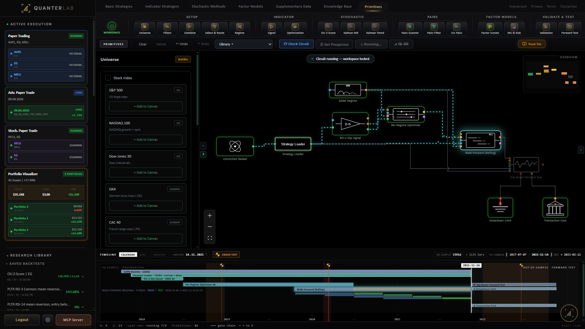
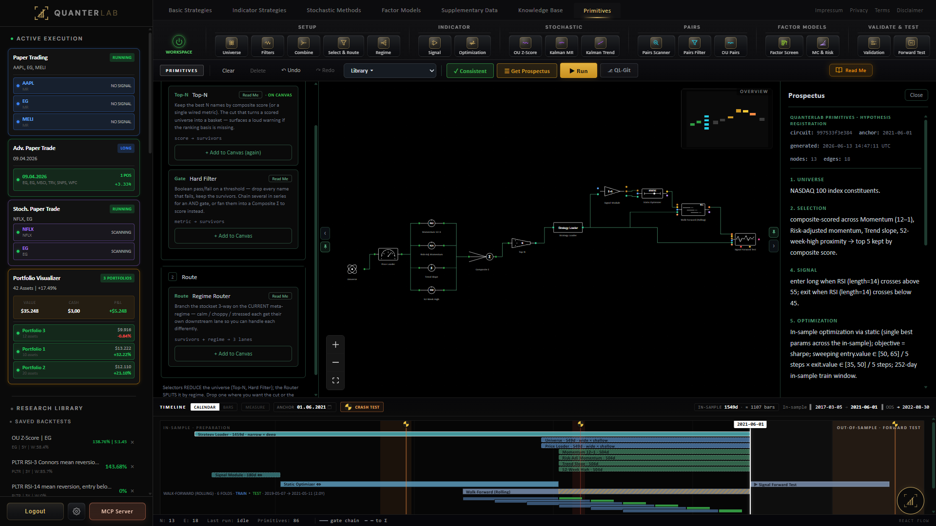
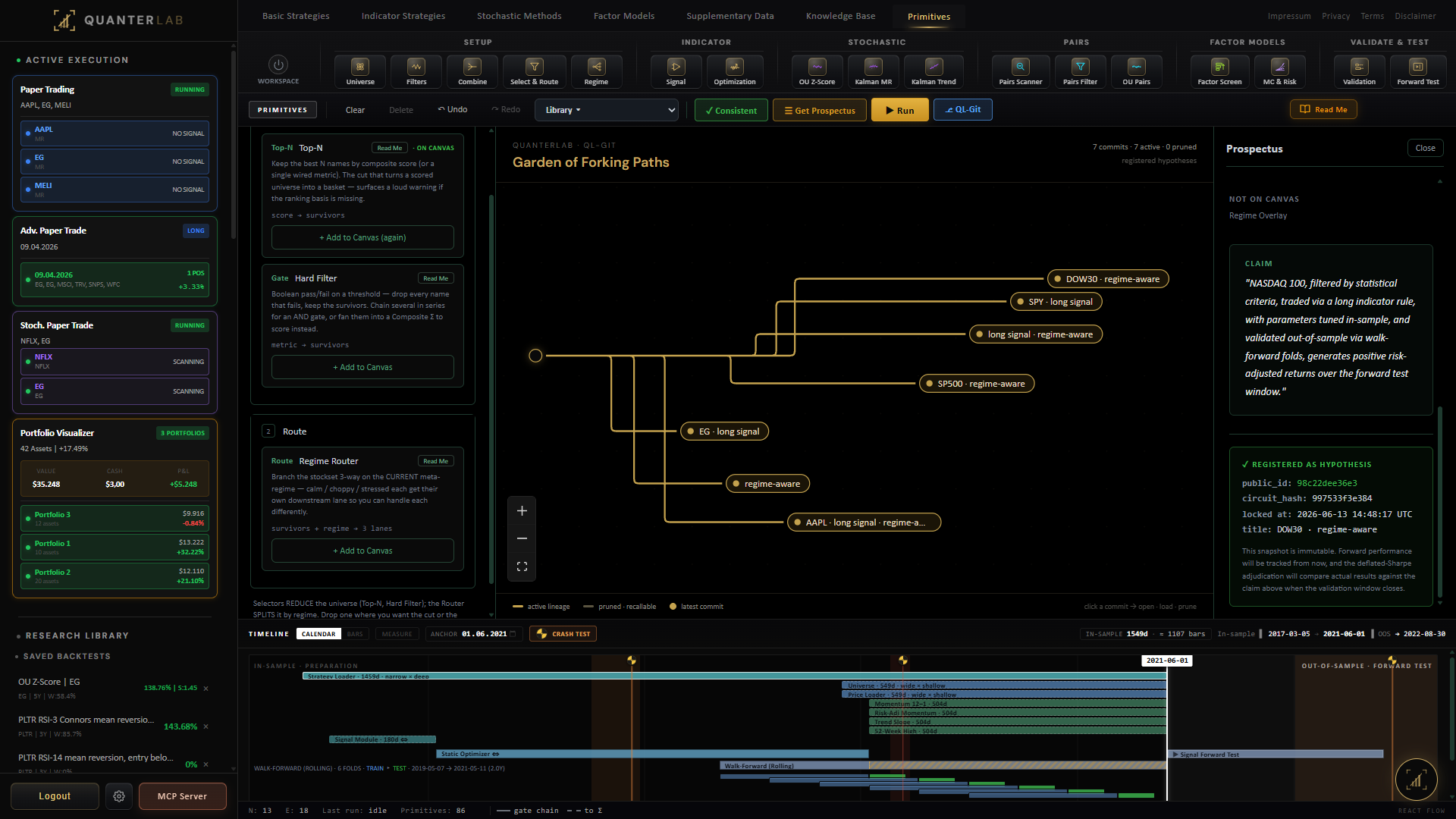
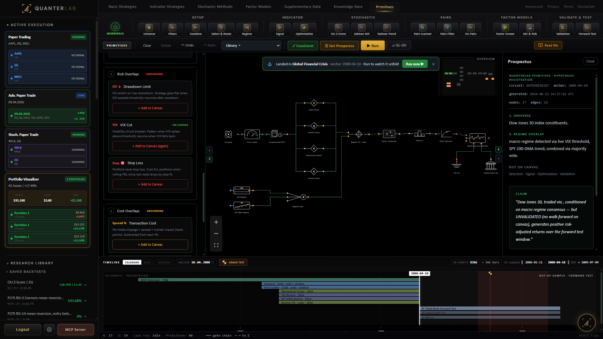
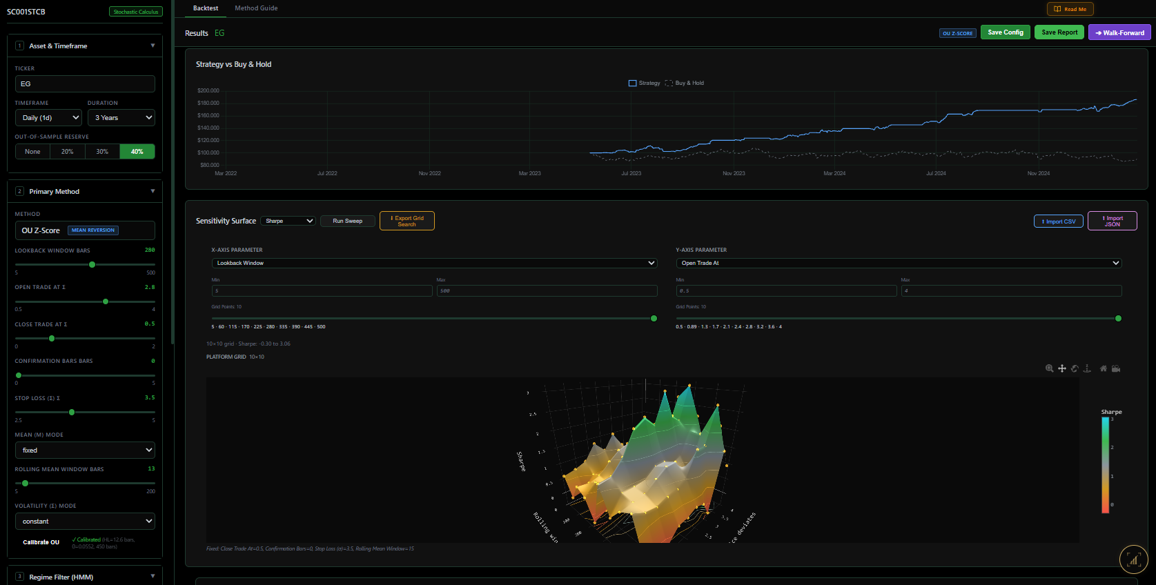
QuanterLab platform — active executions, strategy vs buy-and-hold, sensitivity surfaces
Research Indicators, stochastic methods, factor models — one workflow.
Validation Walk-forward, point-in-time, no survivorship bias.
Execution Paper-trade live; notifies on every fill, daily overnight brief.
Time Travel

Build with what was knowable in 2007. Let the crash decide if you were right in 2008.

Pin a virtual today and the platform replays history forward, bar by bar. The question isn't whether your strategy survives a backtest — it's whether your methodology survives when reality unfolds.

Point-in-time research

Only what existed on the pinned date is visible — universe, constituents, filings, prices. Acting twenty years ago, not fooling yourself with today's survivors.

  • Per-epoch isolation — every artifact stamped with its virtual today
  • Survivorship-corrected universes — delistings included
  • Filings as published — restatements stay in their own epoch
or
Methodology stress test

Build with what was knowable. Replay forward bar by bar — pure methodology, no hindsight in the design.

  • Hermetic builds — nothing from after the cut-off is visible
  • Replay forward — bar by bar, your method on autopilot
  • Market correlation — moved with the tide, or despite it
Pre-loaded crisis cuts
2008
Global Financial Crisis
Drop in at 2007-Q4. Ride the collapse.
2015
China devaluation
Build regime-aware. See what holds when correlations break.
2020
COVID crash
Freeze at 2020-Q1. Test stops, sizing, regime gates.
2022
Rate-hike regime
Strategies that adapted vs those that didn't.
Meet Quantin

Four lenses. One chat thread.

AI assistants agree with you. Quantin's Skeptic doesn't — it probes for curve-fit. The Tutor explains why a step exists. The Librarian reads your saved work. The Mathematician derives the model. Same thread, same data, swap posture per question.

Skeptic · live exchange Example, anonymised
You My backtest got Sharpe 1.62 and 23.47% return on 9 trades. OOS was set to 40%. Ready to deploy?
Quantin Skeptic lens

You haven't run walk-forward. This is fiction.

You set OOS to 40% — good instinct. But you haven't revealed it yet. Your headline numbers — the 1.62 Sharpe, the 23.47% return — are in-sample only. Hypothesis generation. Not validation.

Until you show the OOS Sharpe and the walk-forward decay ratio, you have nothing except evidence that you can fit a curve.

The verdict
Concerning.

All the hallmarks of curve-fit:

  • Tiny trade count
  • Headline Sharpe with no walk-forward validation
  • No instrument specified — could be a universe-wide sweep
  • Parameter optimisation on limited data

Before you trade this or show it to anyone:

  1. Run walk-forward and show the OOS Sharpe. Decay ratio close to 1.0 or the edge is an illusion.
  2. Add 20+ more trades via different thresholds, or accept that you don't have statistical power.
  3. Name the instrument and defend why this edge is specific to it.

If those three hold up, I'll eat my words. Until then: this is a backtest artifact, not a strategy.

Tutor · live exchange Example, anonymised
You What's walk-forward and why does the platform keep nagging me about it?
Quantin Tutor lens

Walk-forward is honesty about the future.

A regular backtest fits parameters on the same window it scores on. That's an in-sample result — the strategy has seen every bar before it traded. Of course it looks good.

Walk-forward slides a rolling window. Fit on the first opt_bars, then trade the next test_bars blind — the strategy has never seen them. Step forward. Repeat. Stitch all those blind segments into one out-of-sample equity curve.

Then check the decay ratio — OOS Sharpe divided by IS Sharpe. Close to 1.0 means the edge survived first contact with the unknown. Far below 1.0 means you fit noise.

Want me to run one now on your last backtest? I can pick sensible defaults for opt / test bars based on your timeframe.

Librarian · live exchange Example, anonymised
You Read my project library. Anything worth picking back up?
Quantin Librarian lens

Three projects worth a second look, one to retire.

I read 18 saved backtests, 4 active projects, 11 trading configs. Three patterns surfaced:

  • Pick back up RSI mean-revert on consumer staples

    Promising tier across four tickers (KO, PG, CL, KMB). You walked away after the first build — OOS Sharpe never decayed below 0.85. Worth running per-regime to see if it survives 2022.

  • Pick back up OU pairs (KO / PEP)

    Half-life under 15 days, beta stable across two epochs. Sitting in “Untitled Project” from April; never got a forward stress test.

  • Investigate Squeeze breakouts on small-cap

    Two configs disagree on direction (long vs short on identical filter output). One of them is wrong — the other is a strong candidate.

  • Retire MACD crossover on QQQ

    Weak tier in five rebuilds across three years. You've optimised this six times; each rebuild looks worse out-of-sample. The data is telling you something.

Want me to open the first one and queue a per-regime optimisation, or shall we start with the contradiction?

Mathematician · live exchange Example, anonymised
You Derive the OU process so I understand what the Stochastic Builder is actually fitting.
Quantin Mathematician lens

Ornstein-Uhlenbeck — mean reversion as a stochastic process.

Start with the continuous-time SDE. The process is pulled back toward its long-run mean \(\mu\) at speed \(\theta\), perturbed by Brownian noise of size \(\sigma\):

\[ dX_t = \theta\,(\mu - X_t)\,dt + \sigma\,dW_t \]

Three parameters, three meanings. \(\theta\) is the speed of reversion — large \(\theta\) snaps back fast. \(\mu\) is the level it reverts to. \(\sigma\) is the noise scale — the width of the band around \(\mu\) the process explores.

From \(\theta\) you get the most actionable quantity, the half-life — the expected time for a deviation from the mean to shrink by half:

\[ t_{1/2} = \frac{\ln 2}{\theta} \]

And the trading signal — the z-score at each bar — is just the standardised deviation from the fitted mean:

\[ z_t = \frac{X_t - \mu}{\sigma / \sqrt{2\theta}} \]

The Stochastic Builder fits \((\theta, \mu, \sigma)\) by maximum likelihood on the discretised AR(1) form. Want me to walk through the AR(1) derivation, or show how the half-life maps to the platform's signal-window control?

Prefer your own AI?

Connect QuanterLab's MCP server to Claude, Codex, or any MCP-compatible client. Your assistant, our research substrate — same point-in-time data, same tools, same boundaries.

Read the MCP docs
Tour the Lab

The research substrate.

The same canonical loop, applied to different primitives — indicator rules, stochastic processes, factor portfolios, paper execution. Drag, swipe, or use the arrows.

Module 01 · Analyse

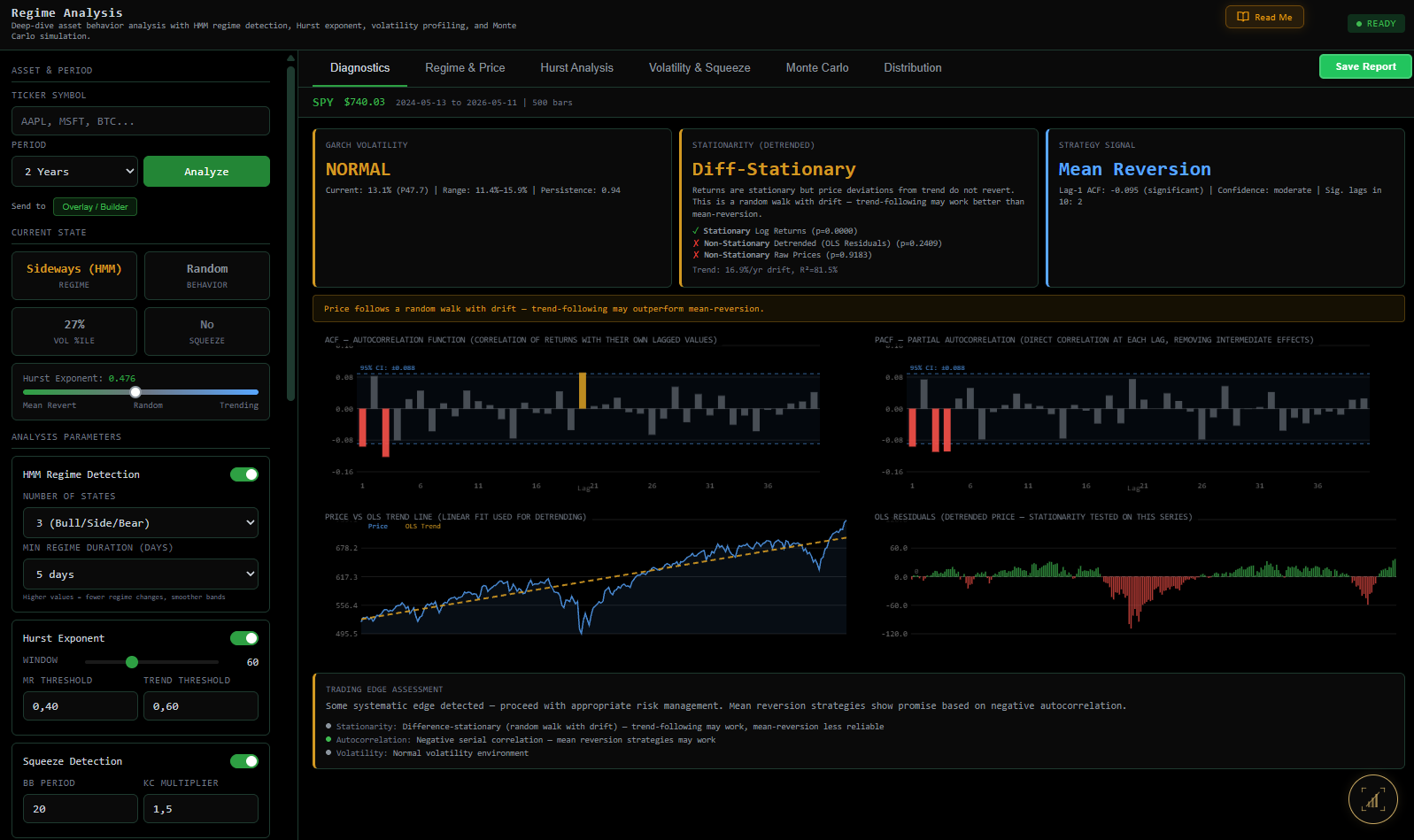
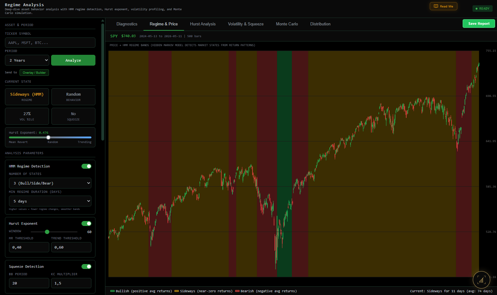
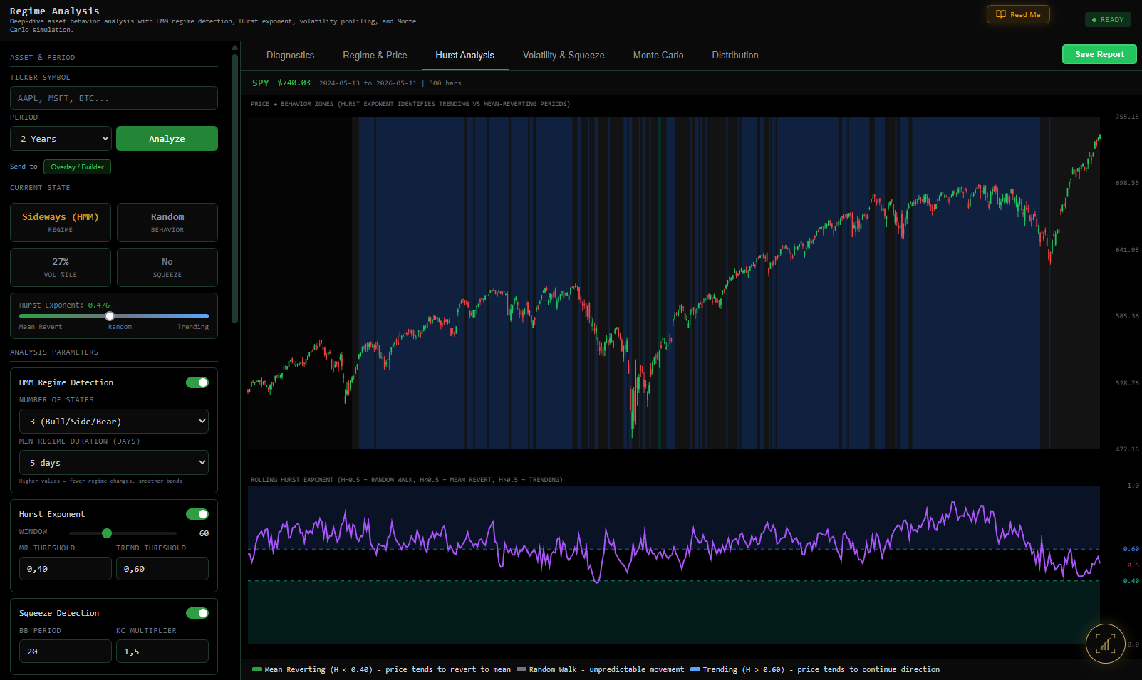
Regime Analysis

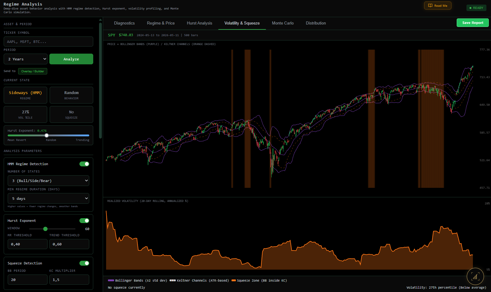
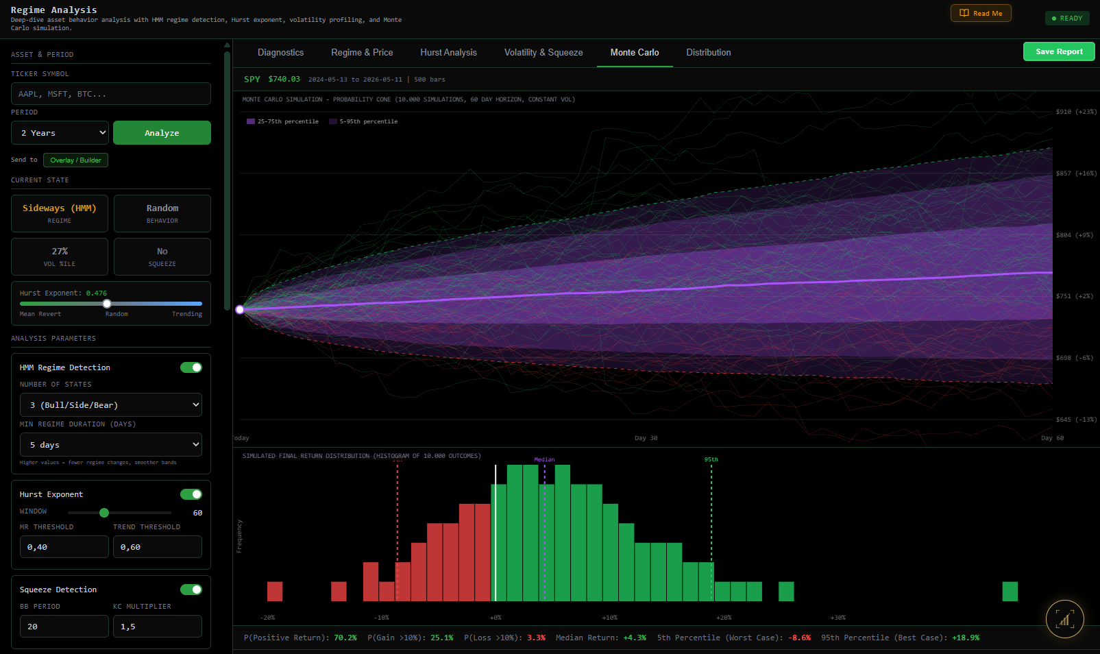
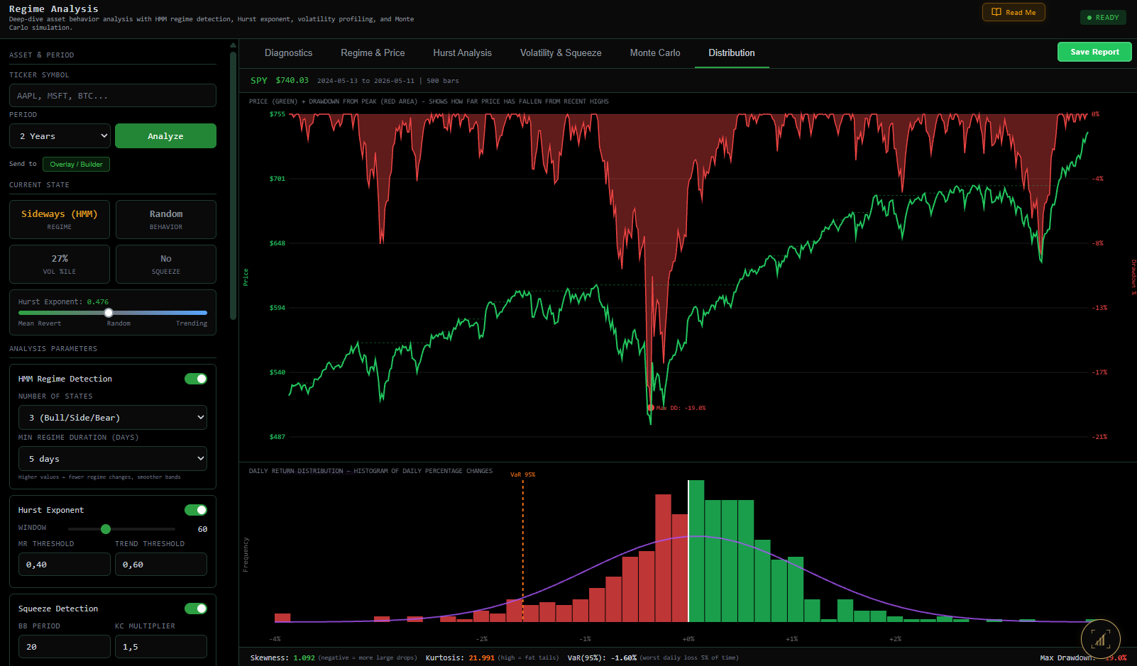
Six diagnostics before you build a rule. Hurst, HMM regimes, volatility squeeze, Monte Carlo, return distribution. If Hurst > 0.5 you're not mean-reverting — the platform tells you so.

Open module
Regime Analysis — Diagnostics
Diagnostics
Regime & Price
Regime & Price
Hurst Analysis
Hurst
Volatility & Squeeze
Vol & Squeeze
Monte Carlo
Monte Carlo
Distribution
Distribution
Modules 02–03 · Build & Optimise

Indicator Strategies — end to end

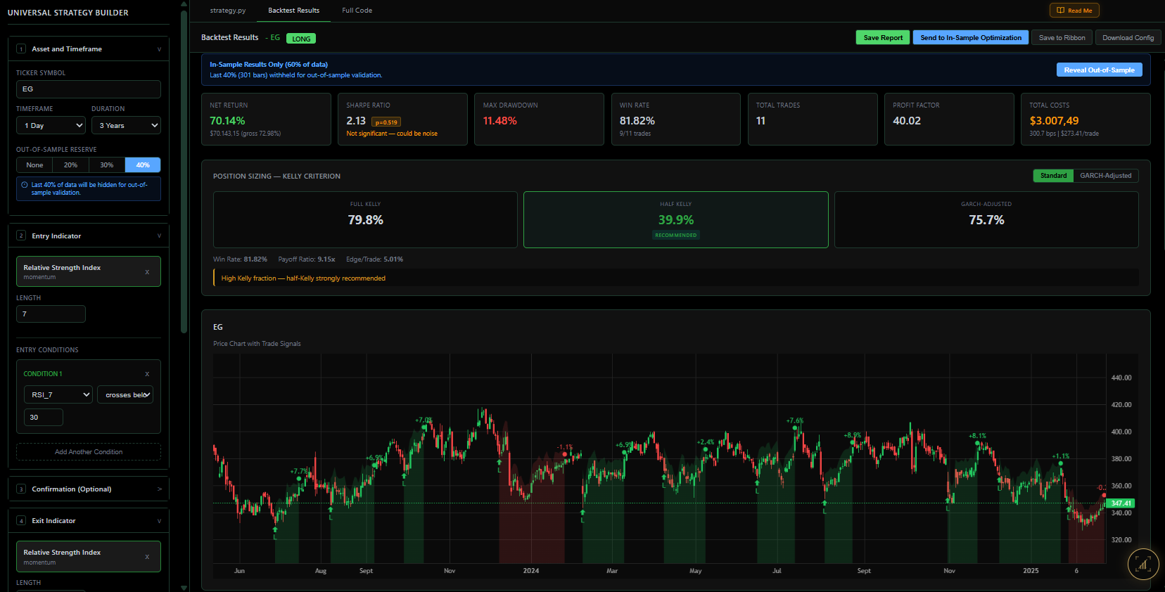
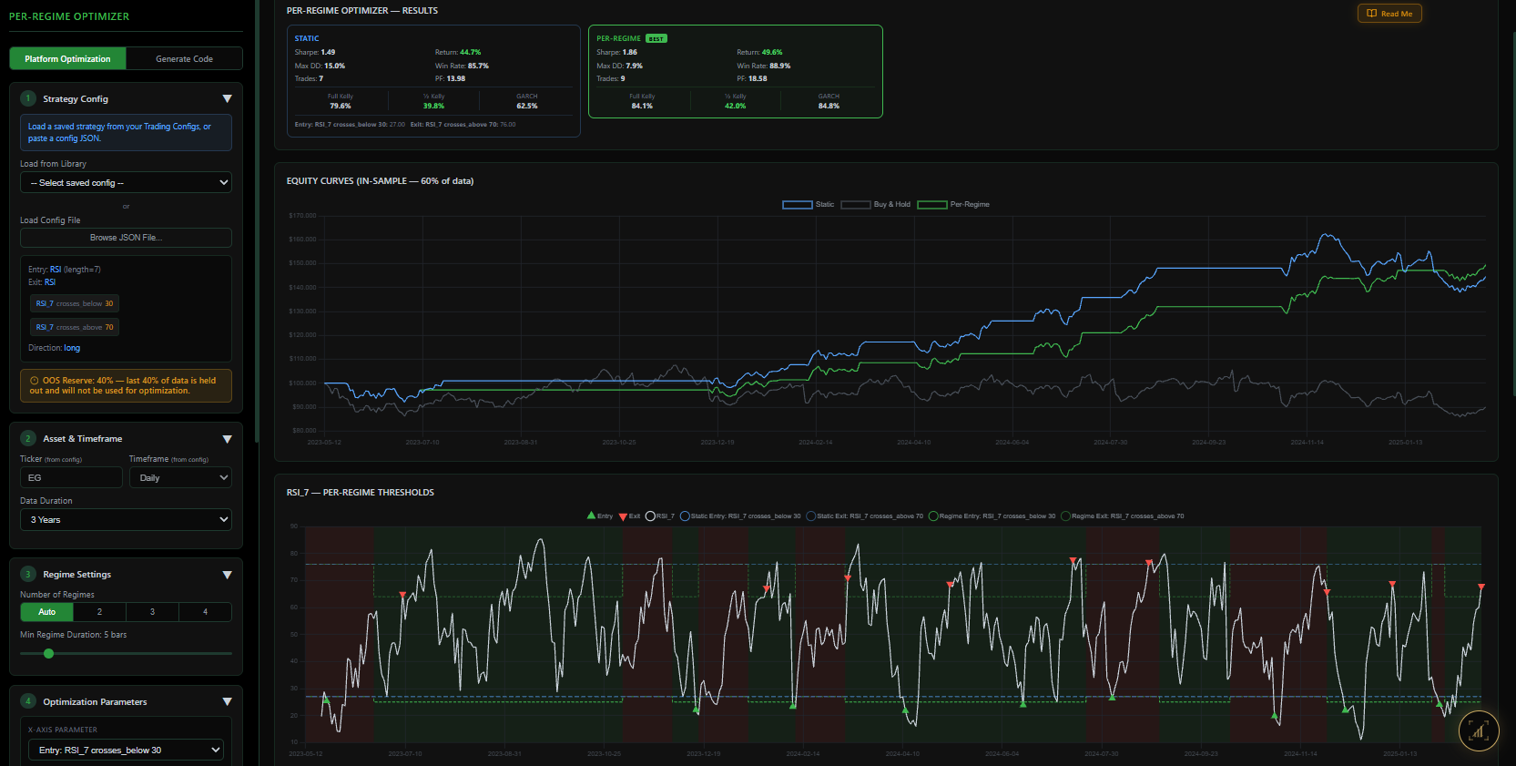
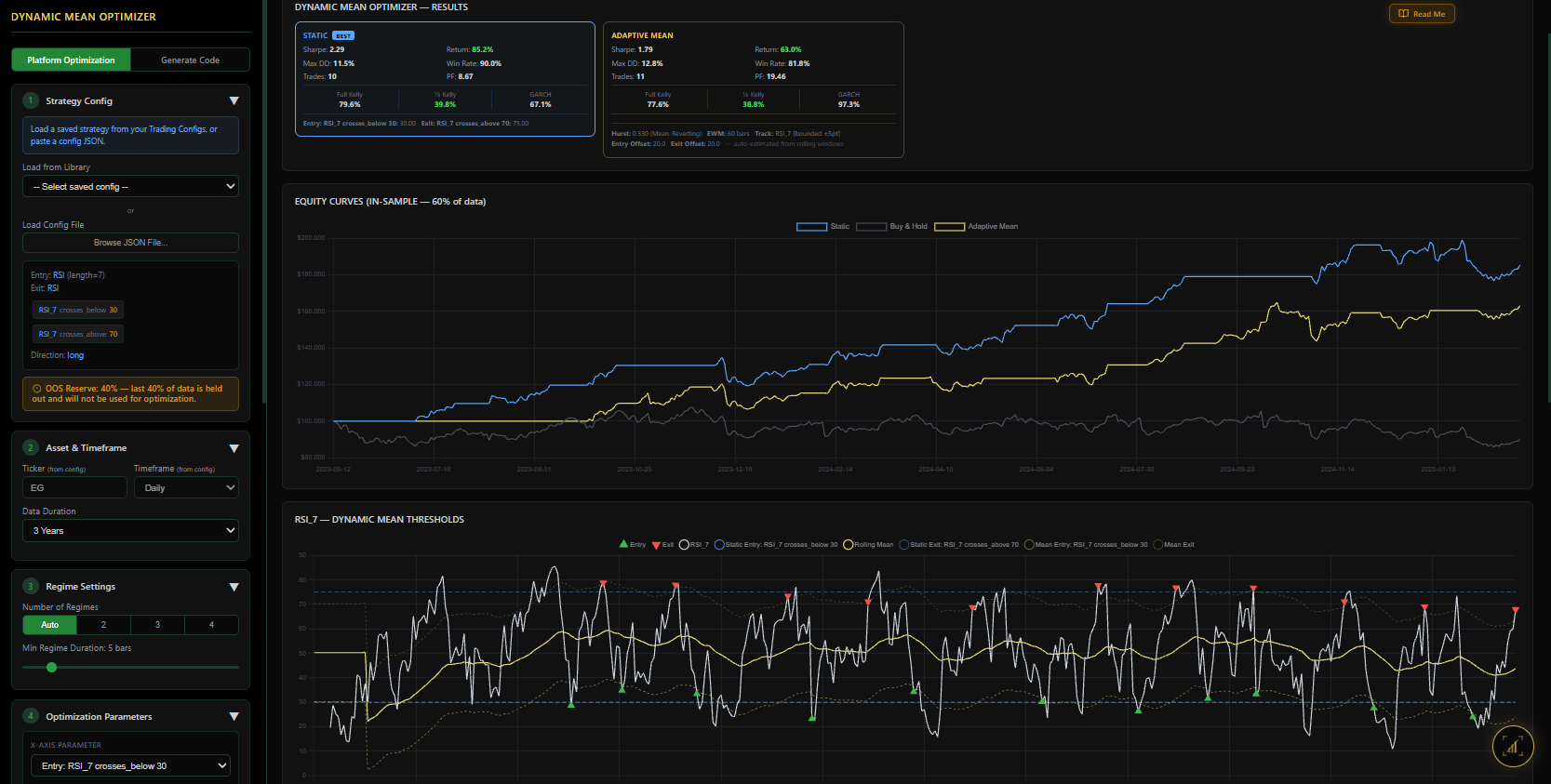
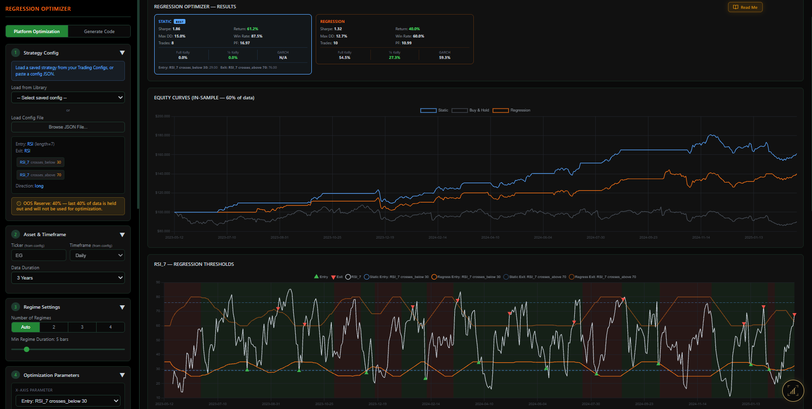
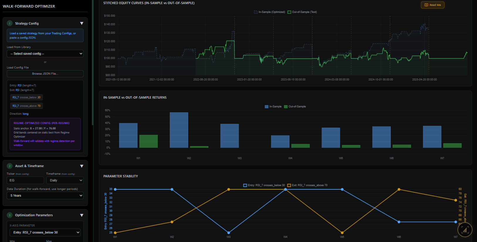
A library of momentum, mean-reversion, crossover and breakout indicators in one builder with up to twenty layers per rule. Four optimisation modes — Static, Per-Regime, Dynamic Mean, Regression — plus walk-forward as the final judge.

Open module
Universal Builder Overlay
Builder Overlay
Per-Regime Optimizer
Per-Regime
Dynamic Mean
Dynamic Mean
Regression Optimizer
Regression
Walk-Forward
Walk-Forward
Module 04 · Stochastic

Stochastic Methods — model the process

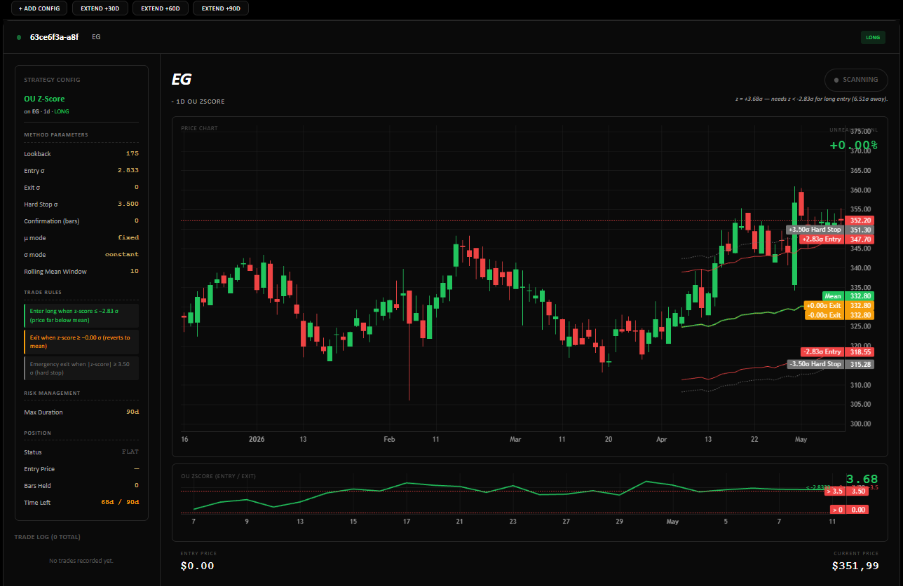
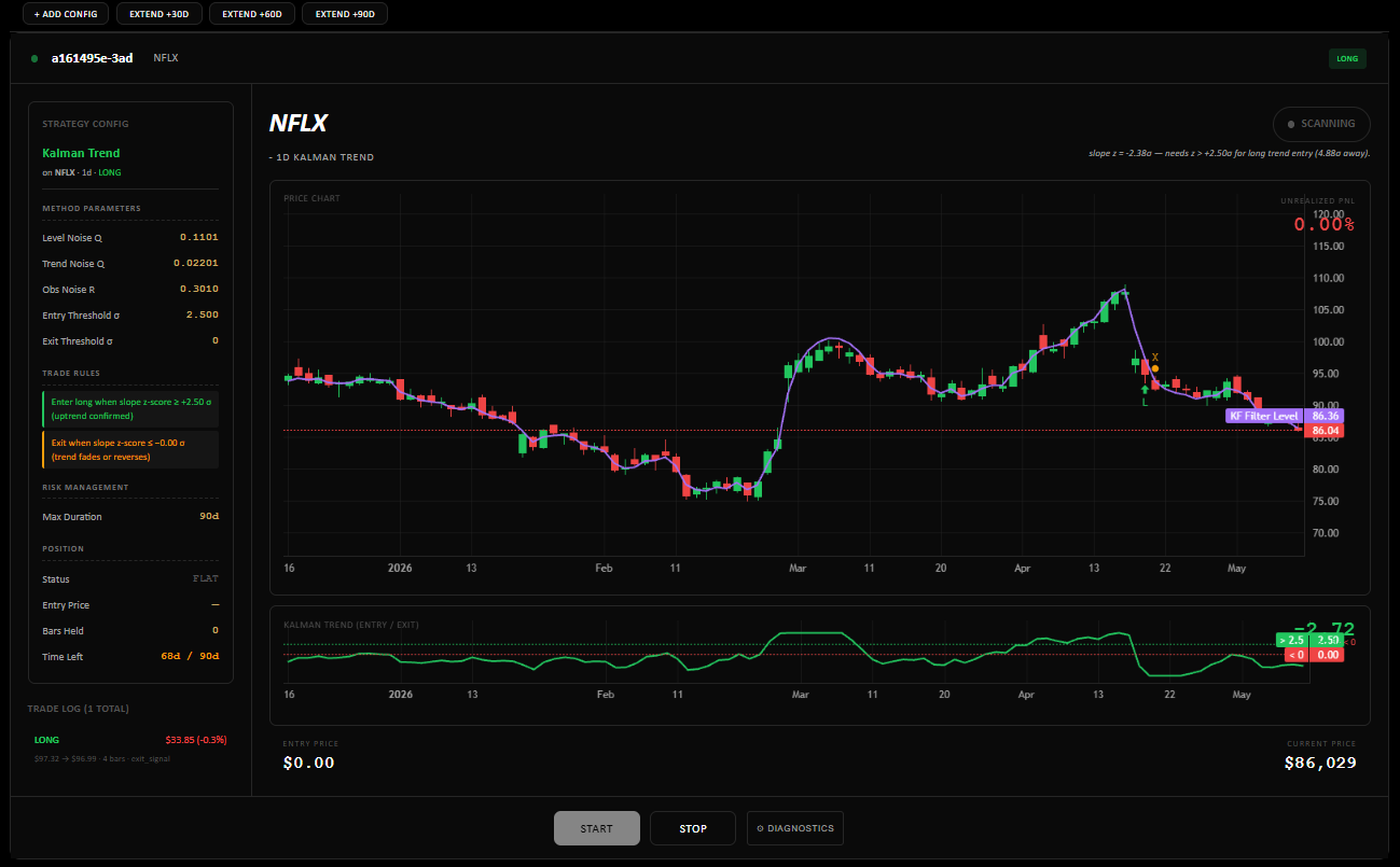
Indicator rules react to symptoms. Stochastic methods describe the underlying process: Ornstein-Uhlenbeck, Kalman, cointegrated pairs, realised volatility surface.

Open module
OU Sensitivity Surface
OU · Sensitivity
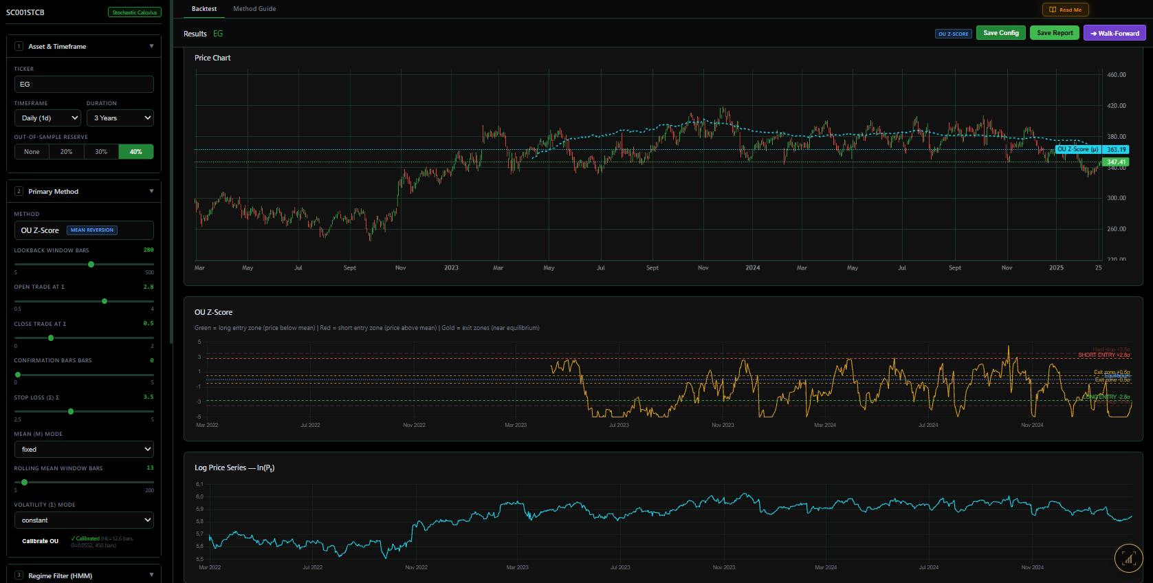
OU Z-Score backtest
OU · Z-Score
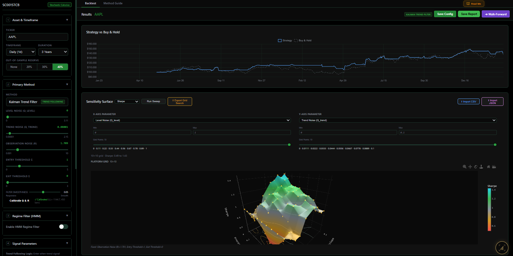
Kalman filter
Kalman
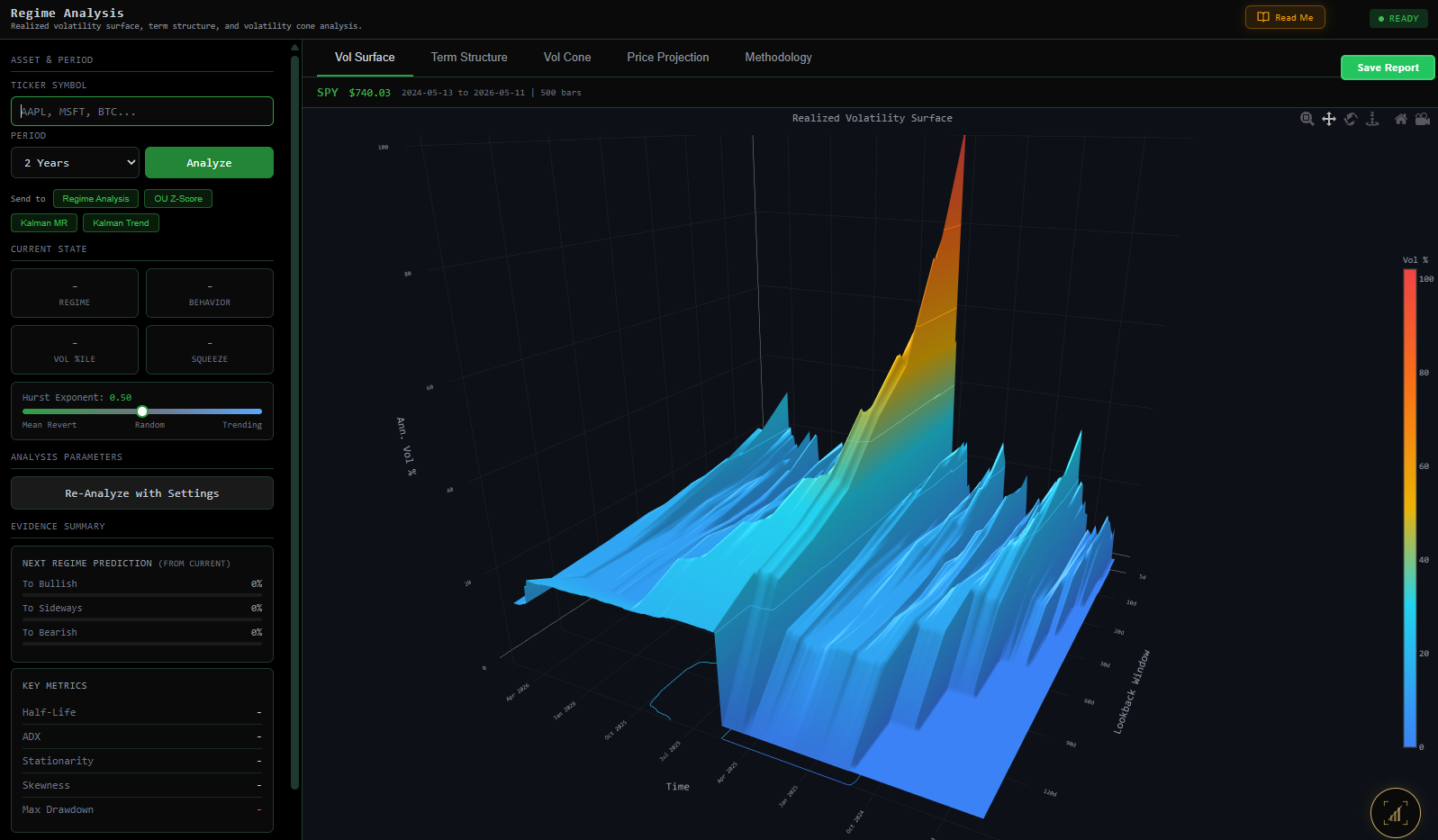
Realised volatility surface
RV Surface
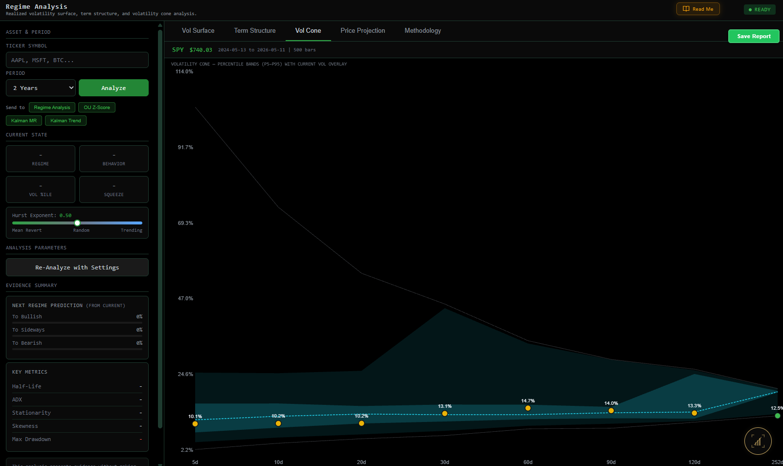
Volatility cone
Vol Cone
Module 05 · Portfolios

Factor Models — portfolios, not trades

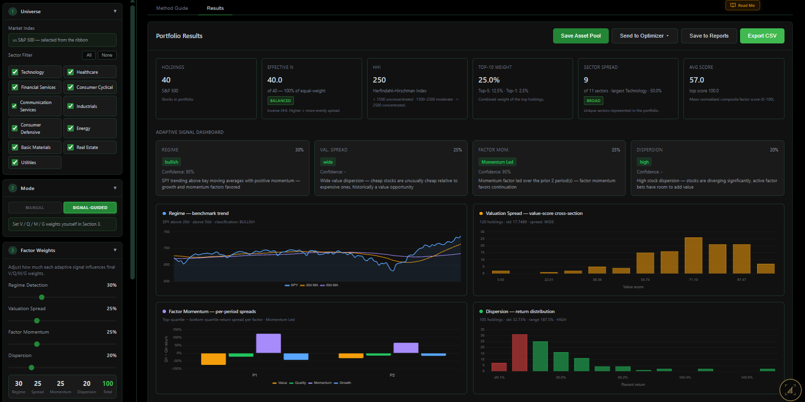
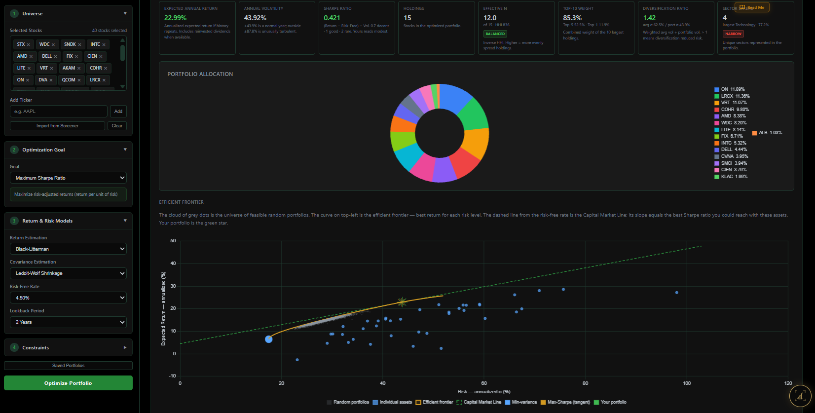
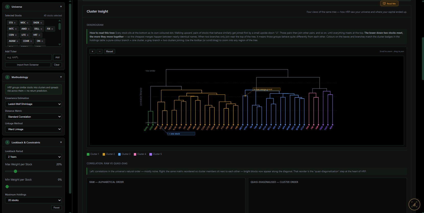
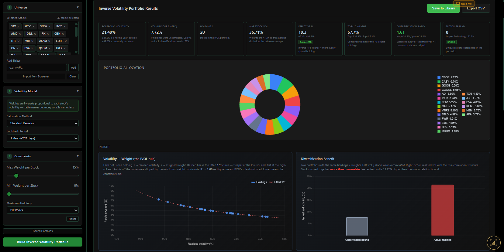
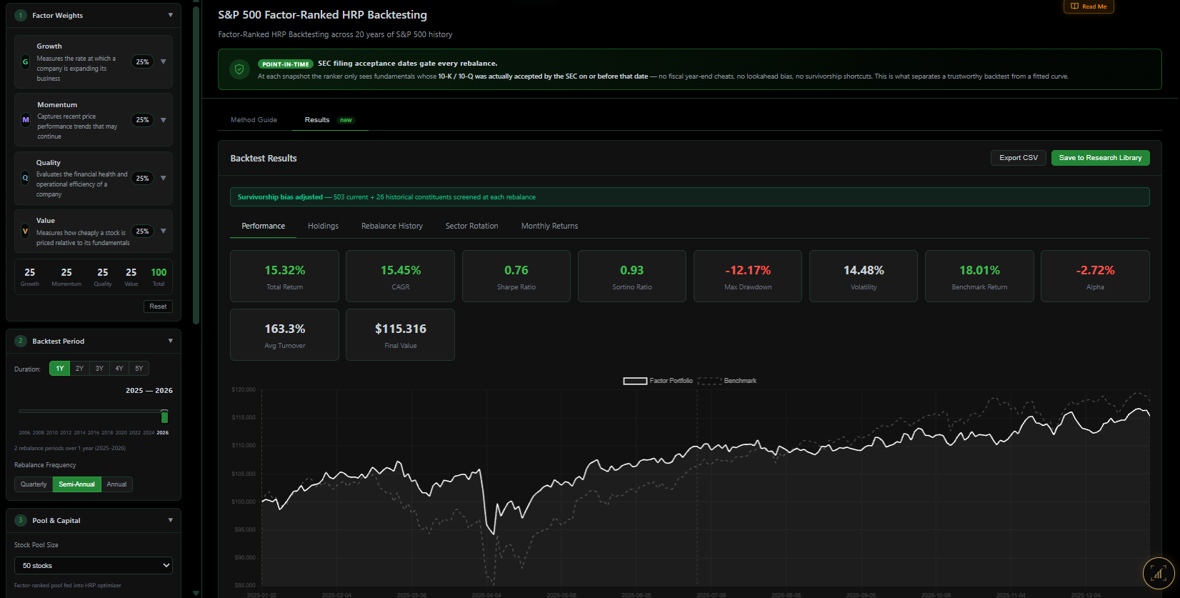
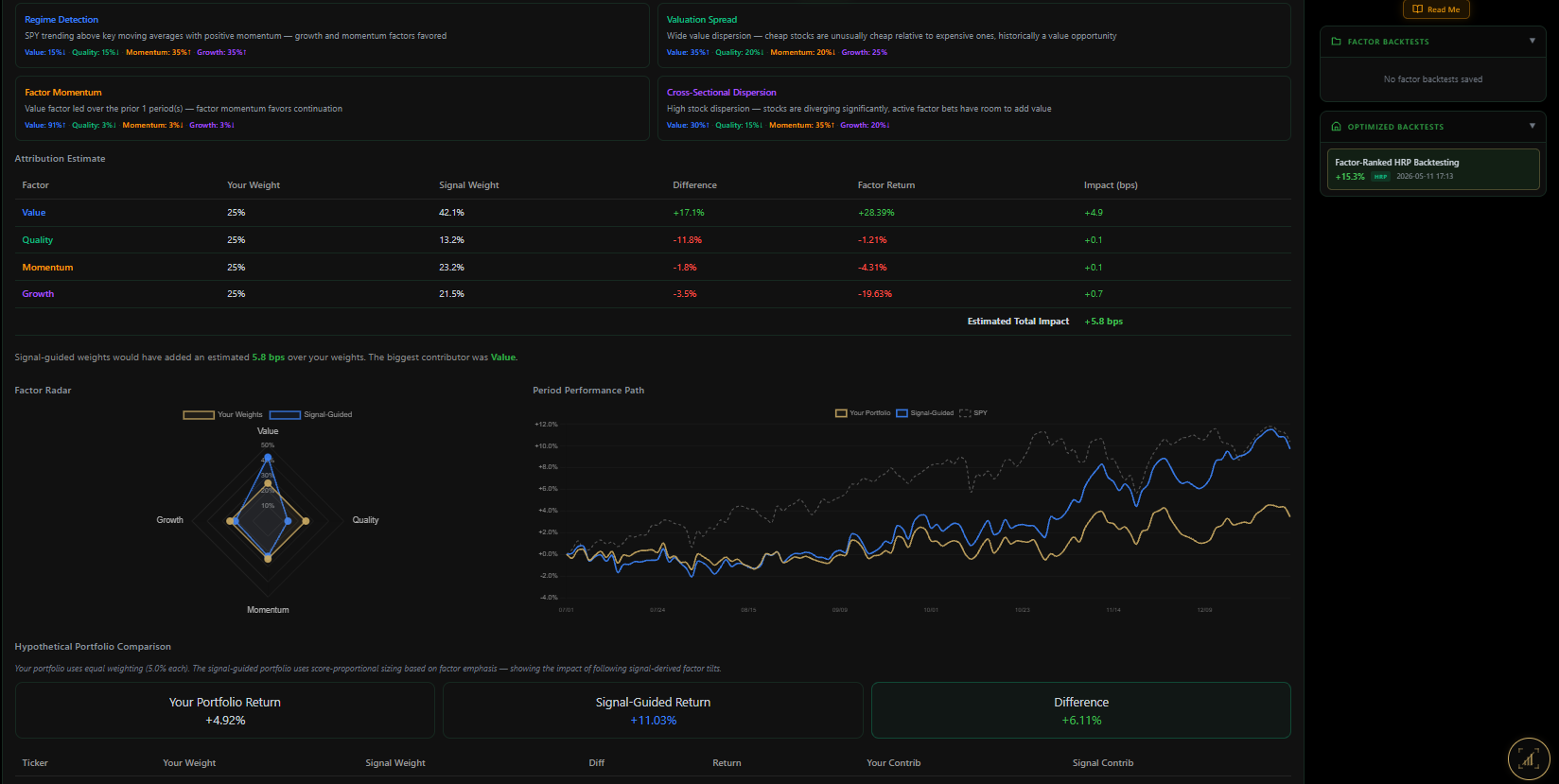
Rank an index by composite factor scores; build a portfolio with MVO / HRP / IVOL; backtest with point-in-time fundamentals; autopsy each rebalance to see which factor carried the run.

Open module
Factor Screener
Screener
MVO
MVO
HRP
HRP
IVOL
IVOL
Portfolio Backtest
Backtest
Autopsy
Autopsy
Cross-cutting · Execution

Paper Trading & Portfolio Visualiser

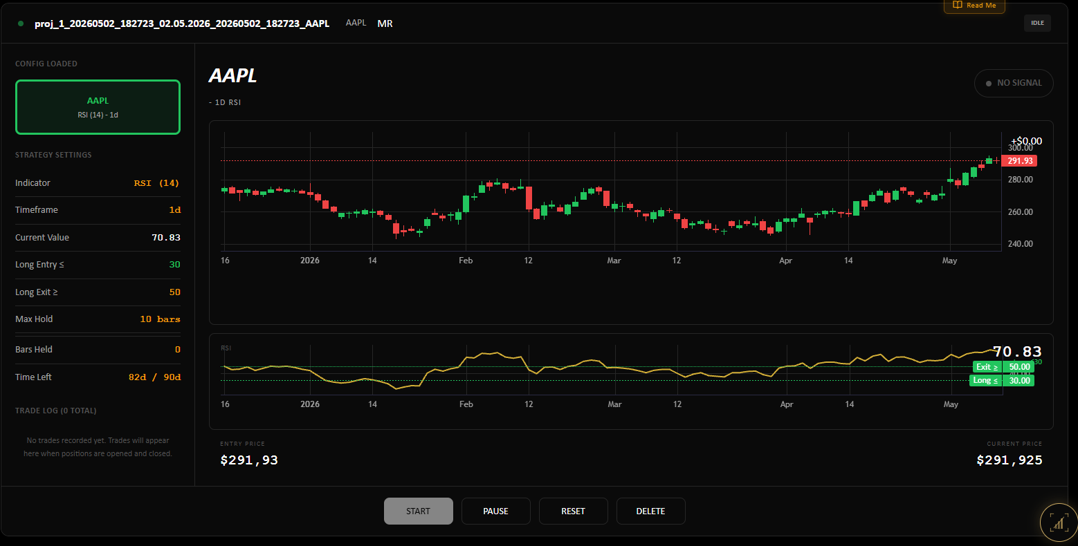
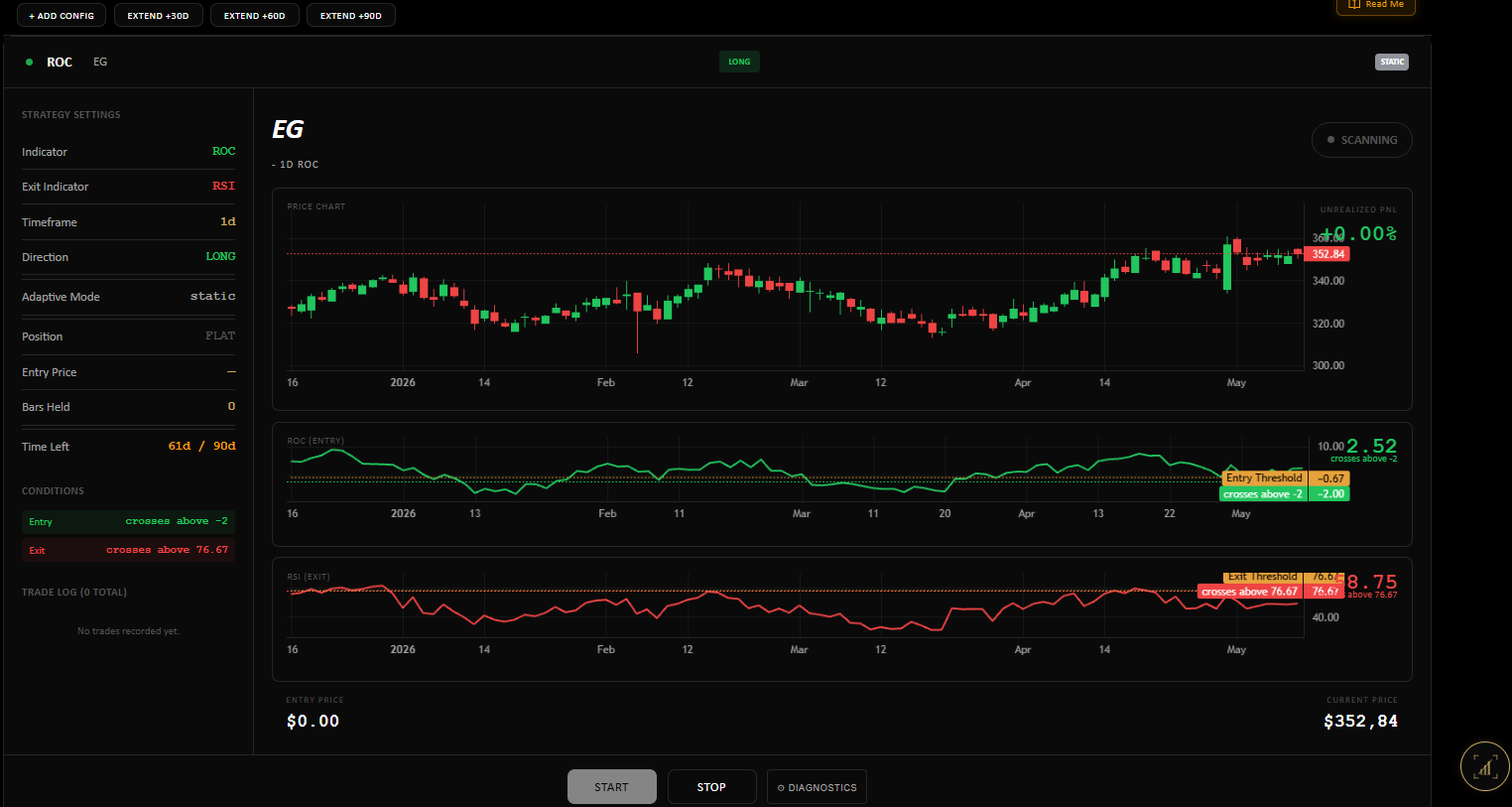
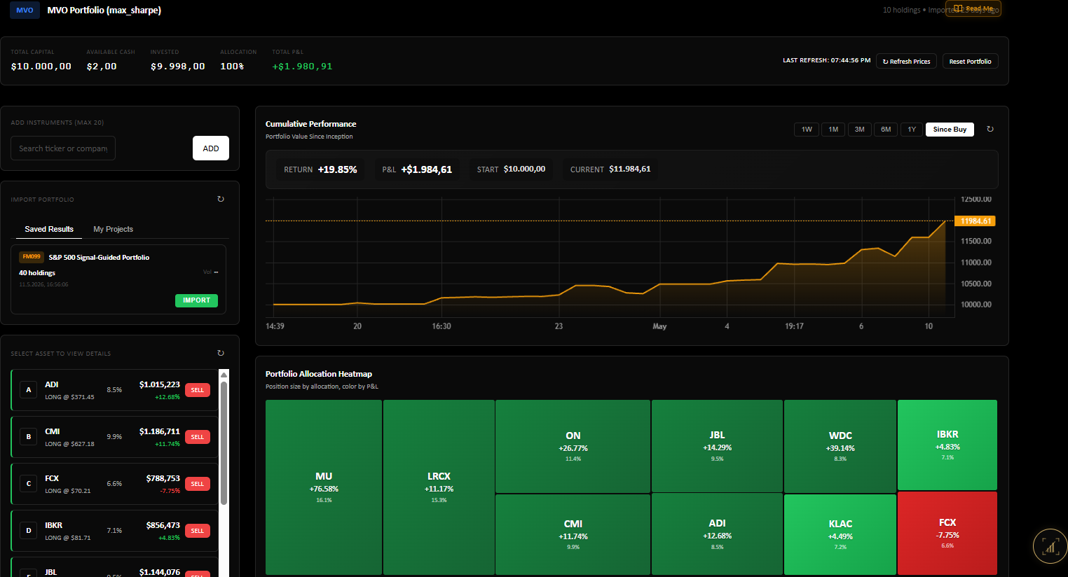
Four paper-trade engines (Basic, Universal, OU, Kalman) — each with its own capital pool, morning brief, and per-trade signal alerts. Plus the Portfolio Visualiser tracks up to three portfolios side-by-side, real-time.

Open module
Basic Paper Trader
Basic
Advanced Paper Trader
Advanced
OU Paper Trader
OU
Kalman Paper Trader
Kalman
Portfolio Visualizer
Portfolio Viewer
Cross-cutting · Code Export

Your code. Your machine. Your scale.

Every backtest, walk-forward, and grid search exports as standalone Python — yfinance + numpy + scipy, no platform deps. Run it on your laptop, scale it on your GPU, drop the JSON output back into the platform viewer.

Download example
1,487
lines of standalone Python
2,500
backtests · 50×50 grid
3
outputs · PNG / CSV / interactive HTML
sc001_NFLX_kalman_trend_grid_50x50.py 1,487 lines
 1  #!/usr/bin/env python3
 2  """
 3  QuanterLab — Grid Search Parameter Optimizer
 4  Generated by QuanterLab on 2026-05-13 19:18
 5  
 6  Runs a 50x50 parameter sweep over:
 7    X-axis: level_covariance (0.0001 to 1)
 8    Y-axis: trend_covariance (1e-05 to 0.1)
 9  
10  Outputs: PNG heatmap + CSV results + interactive HTML 3D
11  Ticker: NFLX  ·  Method: kalman_trend
12  """
13  import yfinance as yf
14  import numpy as np
15  from scipy import stats
16  from statsmodels.regression.linear_model import OLS
17
18  # 50×50 grid — same axes the platform ran
19  LEVEL_COV_GRID = np.logspace(-4, 0, 50)
20  TREND_COV_GRID = np.logspace(-5, -1, 50)
21
22  results = np.zeros((50, 50, 5))  # sharpe, sortino, mdd, …
23  for i, lc in enumerate(LEVEL_COV_GRID):
24      for j, tc in enumerate(TREND_COV_GRID):
25          results[i, j] = backtest(price, lc, tc)
26
27  # 2,500 backtests → CSV + PNG heatmap + 3D HTML viewer
28  np.savetxt("grid.csv", results.reshape(-1, 5), delimiter=",")
29  plot_surface(results, save="grid.html")
30  # Drop grid.html back into QuanterLab's 3D viewer to compare
31  # cloud vs. local. Or scale to 200×200 on your own GPU.
Module 6 · Knowledge Base

Theory and methods, with academic references.

Articles that explain why, not just how. Method deep-dives, conceptual explanations, terminology breakdowns — each grounded in real academic sources you can chase down.

Methodology Why walk-forward is the only validation that counts A backtest that looks great in-sample means nothing if you didn't fold the optimisation step into the validation. What walk-forward actually tests, and what it doesn't. Adaptive Thresholds Per-regime, dynamic mean, regression — when each one wins A side-by-side of the four threshold modes on the same RSI strategy across 2018–2025. Where each mode beats Static, and where it overfits. Falsification The four ways your backtest is lying to you Survivorship bias, look-ahead, restated fundamentals, and the tail-risk you didn't simulate. How Time Travel + bootstrap + Monte Carlo close each gap.

Open the lab.

Free to start. Closed beta — invitation-based.

Create Free Account See Pricing