


O'Shaughnessy's Trending Value Taken Apart: Twenty Years on the S&P 500 as It Stood
Trending Value is a stock-picking formula from James O'Shaughnessy's book "What Works on Wall Street", and stock screeners have copied it for years. It has two components. The value component finds the cheapest stocks in the market, judged on six price measures at once. The trend component then buys, from those cheap stocks, the ones whose prices did best over the last six months.
We wanted to know which component does the work. So we built the formula every January for twenty years, from the companies in the S&P 500 at the time, using only what they had reported by then, and held each year's pick for a year. Beside it we ran two versions, each changing one thing: low P/E as the value component, with the same trend component; and the trend component only, with no value component. We measured each one against the equal-weight S&P 500, with its dividends.
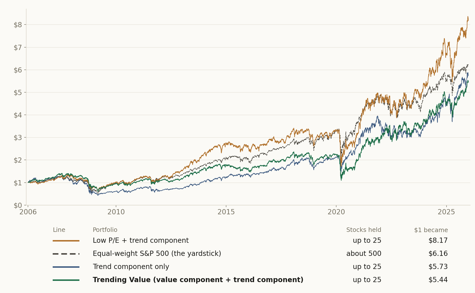
The famous formula made less money than the equal-weight S&P 500, and less than both of its changed versions. The trend component only ended a little ahead of the formula, but fell far deeper in the financial crisis. The change that made a large difference was the value component's measure: with low P/E in place of the six measures, the formula beat the equal-weight S&P 500, and fell less than it in the worst crash.
What Trending Value is
James O'Shaughnessy's book "What Works on Wall Street" is one of the best-known collections of tested stock-picking rules. Its fourth edition added a formula he called Trending Value, and stock screeners have copied it ever since.
The idea behind it is easy to like. A cheap stock can stay cheap for years, so buying cheap alone means a lot of waiting. Trending Value waits for a sign. Its value component first finds the cheapest stocks; its trend component then buys the ones whose prices did best over the last six months, on the view that the market is beginning to agree they were too cheap.
The rules, step by step
The formula has two components:
• The value component: score every stock on six price measures and keep the cheapest tenth, about 50 stocks.
• The trend component: of those, keep the 25 whose prices did best over the last six months. In a falling market these are the ones that fell least.
Every year, on the first trading day of January:
1. Take the companies in the S&P 500 on that day, as the index stood then.
2. The value component. Score each one on six price measures, using only the reports it had filed by then: price to earnings, price to book value, price to sales, enterprise value to EBITDA, the free cash flow yield and the dividend yield. A company losing money counts as expensive on that measure, not cheap. Keep the cheapest tenth.
3. The trend component. Of those, buy the 25 whose prices did best over the last six months, in equal amounts.
4. Hold them for a year with their dividends, then start again.
To see which component does the work, we ran two versions beside it, each changing one thing:
• Low P/E + trend component: the value component on price to earnings alone, keeping the tenth with the lowest price to earnings (a company losing money is never in it), then the same trend component, 25 stocks.
• Trend component only: the 25 stocks that did best over the last six months in the whole index, with no value component.
We measured every portfolio against one yardstick: RSP, the equal-weight S&P 500, with its dividends. It holds every stock in the index in equal amounts and resets them every quarter; our portfolios start each year in equal amounts and are then left alone.
What we found, in short
Did Trending Value beat the equal-weight S&P 500? No (Figure 1). For the first years it kept pace, through the crash and the recovery after it. Then came the long stretch when cheap stocks were out of favour almost everywhere, and the formula fell far behind. It won part of that back near the end, but it never caught up.
Does the value component matter? For where the money ended, very little (Figure 1). The trend component only, buying the stocks that had done best with no regard for price, ended a little ahead of Trending Value. The ride was the difference: in the financial crisis these stocks fell the furthest of all, and they took years to climb back.
Do six measures beat one? No, and this was the surprise (Figure 1). With low P/E as the value component and the same trend component after it, the formula stayed close to Trending Value until the financial crisis, then pulled ahead and never fell behind again.
Did any version beat the equal-weight S&P 500? Yes, one (Figure 1). Low P/E + trend component ended with more money, and in the worst crash it fell less. It pulled ahead in the years after the financial crisis, lost the lead for a while in the pandemic crash, and finished the twenty years further ahead than ever.
1 Methodology, in detail (click to open)
1 Methodology
Universe: the S&P 500's members on each first trading day of January from 2006 to 2025, rebuilt from the index's change log. Fundamentals: each company's statements as filed with the SEC, visible only from the day they were accepted. Value component: the platform's Value Factor card with six measures at equal weight, scored as percentiles across the index, cut to the cheapest tenth; its setting for a negative multiple ranks a loss, a negative book or a negative EBITDA as the most expensive. Trend component: the Momentum Factor card's six-month price change, the latest month included, ranked within that tenth, the top 25 kept. Portfolio: equal weights, bought at the first close of the year and held to its last close, dividends reinvested on their ex-dates, 10 basis points paid on each purchase and each sale. RSP is held the same way, with its dividends and no costs, from each year's first close to its last, so, as for every portfolio here, the move into each year's first trading day is left out; held without that gap, $1 in RSP became $6.68. Each year was written down and locked before it ran.
2 Results
Findings
Table 1 sets the four side by side over the twenty years.
2.1 Headline
Table 1. Ups and downs a year: the standard deviation of daily returns, annualised. Sharpe ratio: the average yearly return divided by those ups and downs, before any cash rate. Dividends reinvested, 10 basis points paid at entry and at exit. RSP, the equal-weight S&P 500, is bought at each year's first close and held to its last, with its dividends and no costs.
| Portfolio | $1 became | A year | Worst fall | Ups and downs a year | Sharpe ratio |
|---|---|---|---|---|---|
| Low P/E + trend component | $8.17 | 11.1% | −54% | 23.3% | 0.57 |
| Equal-weight S&P 500 (the yardstick) | $6.16 | 9.5% | −61% | 20.7% | 0.54 |
| Trend component only | $5.73 | 9.1% | −67% | 25.1% | 0.47 |
| Trending Value (value component + trend component) | $5.44 | 8.8% | −57% | 22.7% | 0.49 |
Sections 2.2 to 3, the full record: every year, every test, and how each one was run (click to open)
The registration names the two groups compared Trending Value and The same rule on price to earnings alone; this paper calls them Trending Value and Low P/E + trend component.
2.2 Per-step results
| # | Out-of-sample window | Trending Value SR | Low P/E + trend component SR | Trend component only SR |
|---|---|---|---|---|
| 1 | 2006-01-03 → 2006-12-29 | 1.39 | 0.87 | 0.74 |
| 2 | 2007-01-03 → 2007-12-31 | 0.76 | 1.03 | -0.10 |
| 3 | 2008-01-02 → 2008-12-31 | -1.14 | -0.86 | -0.86 |
| 4 | 2009-01-02 → 2009-12-31 | 0.59 | 0.83 | 0.26 |
| 5 | 2010-01-04 → 2010-12-31 | 0.62 | 0.79 | 0.86 |
| 6 | 2011-01-03 → 2011-12-30 | 0.27 | 0.19 | -0.30 |
| 7 | 2012-01-03 → 2012-12-31 | 0.63 | 1.73 | 1.12 |
| 8 | 2013-01-02 → 2013-12-31 | 2.34 | 2.45 | 2.23 |
| 9 | 2014-01-02 → 2014-12-31 | 0.53 | 1.26 | 0.93 |
| 10 | 2015-01-02 → 2015-12-31 | -0.52 | -0.21 | 0.66 |
| 11 | 2016-01-04 → 2016-12-30 | 1.36 | 0.72 | 0.91 |
| 12 | 2017-01-03 → 2017-12-29 | 1.21 | 0.98 | 1.44 |
| 13 | 2018-01-02 → 2018-12-31 | -0.86 | -0.85 | -0.45 |
| 14 | 2019-01-02 → 2019-12-31 | 1.64 | 1.53 | 2.20 |
| 15 | 2020-01-02 → 2020-12-31 | 0.05 | 0.15 | 0.83 |
| 16 | 2021-01-04 → 2021-12-31 | 1.62 | 1.72 | 1.50 |
| 17 | 2022-01-03 → 2022-12-30 | 0.67 | -0.15 | -0.64 |
| 18 | 2023-01-03 → 2023-12-29 | 0.73 | 1.08 | 1.05 |
| 19 | 2024-01-02 → 2024-12-31 | 1.12 | 1.29 | 1.29 |
| 20 | 2025-01-02 → 2025-12-31 | 1.00 | 0.96 | 1.12 |
2.3 Search accounting
No search record exists for this design. It was not promoted from a recorded evolving search, so the number of alternatives tried before it, on paper, in another tool, or in the author's head, is unknown. Unknown is a different fact from one: a study with no lineage is not a strategy with one trial, it is a strategy with an unrecorded number of them. Accordingly no count of alternatives tried is claimed, and nothing in this paper is corrected for a search that was never recorded; the number that stands is the raw out-of-sample result plus this disclosure. The registered per-step record below (§4) still guarantees each window's hypothesis was hashed and registered before that window was scored.
2.4 The comparison
Both arms trade the same registered windows, so their returns can be PAIRED: inside each window the two return series are inner-joined date by date and the difference rTrending Value − rLow P/E + trend component is the object under test. Because this is ONE pre-declared contrast, frozen at registration before any window was scored, the paired statistic needs no multiple-testing deflation, and the per-arm pooled numbers above are likewise uncorrected, because this design has no recorded search to correct against (§2.3). The paired contrast carries that gap differently from the arm levels: it was declared before each window ran and it is scored on the difference, so no window could be read first and scored after. What the timestamps cannot speak to is how this contrast came to be the declared one, which is the limit §2.3 states.
In the table: Arm A = Trending Value · Arm B = Low P/E + trend component.
| # | Window | Paired bars | Arm A | Arm B | Δ | Leader | Trend component only |
|---|---|---|---|---|---|---|---|
| 1 | 2006-01-04 → 2006-12-29 | 250 | +20.4% | +10.6% | +9.8 pp | Arm A | +14.4% |
| 2 | 2007-01-04 → 2007-12-31 | 250 | +12.9% | +18.5% | -5.6 pp | Arm B | -3.7% |
| 3 | 2008-01-03 → 2008-12-31 | 252 | -37.8% | -36.1% | -1.7 pp | Arm B | -46.5% |
| 4 | 2009-01-05 → 2009-12-31 | 251 | +11.9% | +20.7% | -8.8 pp | Arm B | +3.5% |
| 5 | 2010-01-05 → 2010-12-31 | 251 | +11.4% | +16.1% | -4.7 pp | Arm B | +23.0% |
| 6 | 2011-01-04 → 2011-12-30 | 251 | +3.5% | +1.5% | +2.1 pp | Arm A | -14.5% |
| 7 | 2012-01-04 → 2012-12-31 | 249 | +7.8% | +30.2% | -22.4 pp | Arm B | +15.2% |
| 8 | 2013-01-03 → 2013-12-31 | 251 | +41.8% | +48.7% | -6.9 pp | Arm B | +45.4% |
| 9 | 2014-01-03 → 2014-12-31 | 251 | +7.3% | +19.5% | -12.2 pp | Arm B | +16.1% |
| 10 | 2015-01-05 → 2015-12-31 | 251 | -9.1% | -4.6% | -4.5 pp | Arm B | +10.6% |
| 11 | 2016-01-05 → 2016-12-30 | 251 | +20.2% | +10.7% | +9.5 pp | Arm A | +12.8% |
| 12 | 2017-01-04 → 2017-12-29 | 250 | +14.7% | +13.1% | +1.6 pp | Arm A | +22.6% |
| 13 | 2018-01-03 → 2018-12-31 | 250 | -15.9% | -15.5% | -0.4 pp | Arm B | -10.7% |
| 14 | 2019-01-03 → 2019-12-31 | 251 | +20.8% | +21.5% | -0.7 pp | Arm B | +26.8% |
| 15 | 2020-01-03 → 2020-12-31 | 252 | -10.3% | -3.8% | -6.5 pp | Arm B | +26.5% |
| 16 | 2021-01-05 → 2021-12-31 | 251 | +44.8% | +48.8% | -4.0 pp | Arm B | +38.5% |
| 17 | 2022-01-04 → 2022-12-30 | 250 | +14.7% | -6.8% | +21.4 pp | Arm A | -18.7% |
| 18 | 2023-01-04 → 2023-12-29 | 249 | +12.8% | +20.5% | -7.7 pp | Arm B | +16.4% |
| 19 | 2024-01-03 → 2024-12-31 | 251 | +20.7% | +24.6% | -4.0 pp | Arm B | +25.6% |
| 20 | 2025-01-03 → 2025-12-31 | 249 | +20.0% | +22.9% | -2.9 pp | Arm B | +30.1% |
Paired Sharpe of the difference track: -0.31 · block bootstrap (2000 paths, block 10, seed 1234): P(Trending Value beats Low P/E + trend component) = 7.0%.
Window win-rate. Trending Value led 5 of 20 windows (25.0%), Low P/E + trend component led 15, and the mean window gap of -2.43 pp points the same way. Widest single window: 2012 at -22.4 pp.
3 The circuit
The strategy is a circuit of platform primitives, frozen when the study is registered. Below is the circuit as wired on the canvas, the objective it encodes and how the search runs through it, followed by the mathematics each primitive actually computes, the same formulas the execution engine runs. The complete parameterisation is preserved in the study ledger (Appendix A).
The sentence below is the registration record, generated when the circuit was registered and printed verbatim; the authored description of the design is Section 1.
A COMPARATIVE study: Trending Value vs The same rule on price to earnings alone, walked on the same registered out-of-sample windows. Trending Value: S&P 500, bought equal weight at the anchor close and held one year, and run out-of-sample from the anchor: anything the design estimates from history, where it estimates at all, is re-estimated at each anchor from pre-anchor data only, and the walk advances through registered out-of-sample windows; its disposition is the realized forward path versus the benchmark. The same rule on price to earnings alone: S&P 500, bought equal weight at the anchor close and held one year, and run out-of-sample from the anchor: anything the design estimates from history, where it estimates at all, is re-estimated at each anchor from pre-anchor data only, and the walk advances through registered out-of-sample windows; its disposition is the realized forward path versus the benchmark. The arms differ in: Value Factor, Dividend Yield: medium → off; Value Factor, EV/EBITDA: medium → off; Value Factor, FCF Yield: medium → off; Value Factor, P/B Ratio: medium → off; Value Factor, P/S Ratio: medium → off. The contrast under test: whether Trending Value generates better risk-adjusted returns than The same rule on price to earnings alone over the identical out-of-sample windows.
Every block in this study is a card from the platform's catalog: the S&P 500 as it stood on each day, the Fundamentals Loader, the Value Factor with six measures, the Factor Composite and Factor Select for the cheapest tenth, the Momentum Factor on the six-month rise and a second Factor Select for the 25, and the Held Forward Test for the year. You can rebuild every test and change any setting.
Envelopes show counts, ratios, dates, and the parameters the author chose. Full price and per-name data series are not republished: the underlying market data is licensed to QuanterLab. Point figures quoted in the prose, a named holding's return over a stated span, are summary facts derived from public market prices, not redistributed series.
The objective and the search
Trending Value
| Universe | S&P 500 index constituents. |
|---|---|
| Validation & out-of-sample | held forward test (every wired name bought equal weight at the anchor close and held to the end of the one year window, dividends reinvested on the ex-date, 10 basis points one way at entry and at exit, fewer than 10 names excludes the window, SPY held the same way as the benchmark). |
| Other components | Factor models: Factor Composite ×2, Factor Select ×2, Fundamentals Loader (PIT) ×2, Momentum Factor, Value Factor. |
The same rule on price to earnings alone
The specification is identical to Trending Value's table above, row for row; the one registered difference between the arms is itemized below.
What differs between the arms, one manipulated variable, expressed as 5 paired settings on one node:
- paramValue Factor, Dividend Yield: medium → off
- paramValue Factor, EV/EBITDA: medium → off
- paramValue Factor, FCF Yield: medium → off
- paramValue Factor, P/B Ratio: medium → off
- paramValue Factor, P/S Ratio: medium → off
Companion book. Trend component only comes from a companion run of the identical configuration on its own registered anchor schedule. Its results run through this paper's tables under its own name.
Everything else is held identical, so an out-of-sample gap between the arms is attributable to this one change.
Cost elements are wired into the circuit, the realised drag is reported per step in Appendix B.
Show the mathematics, 7 primitives, formulas and parity notes
3.1 Universe
The starting set of tickers, resolved point-in-time from the index change-log, so names delisted or removed later still compete on the dates they traded.
Before any math, you need a list of stocks. An index preset (S&P 500, Nasdaq-100, Dow 30) is reconstructed as it stood ON your anchor date by replaying the historical add/drop change-log backwards, so a 2018 backtest sees the 2018 membership, not today's winners.
Start from today's constituents and un-apply every membership change after the anchor t:
\mathcal{U}(t) = \mathcal{U}_{\text{now}} \;\ominus\; \{\text{adds after } t\} \;\oplus\; \{\text{drops after } t\}3.2 Factor Loader
Point-in-time fundamentals, never let the user see a number before the SEC did.
Loads ~23 fundamental metrics (valuation, quality, growth) per name, but with one inviolable rule: a financial statement becomes visible only on or after its SEC acceptedDate. A 2020 backtest sees only what was actually filed by 2020, no look-ahead, ever.
\text{visible}(f, t) \iff \text{acceptedDate}(f) \le t3.3 Factor Value
Value, how cheap is the stock, cross-sectionally?
Blends cheapness metrics, P/E, P/B, P/S, EV/EBITDA (lower is better) plus free-cash-flow and earnings yields (higher is better). Each metric is z-scored across the universe, winsorized against outliers, weighted by the importance you set (Off/Low/Med/High), and averaged.
z_{i,k} = \pm\,\frac{x_{i,k} - \bar x_k}{s_k}\text{Value}_i = \frac{\sum_k \omega_k\,z_{i,k}}{\sum_k \omega_k}, \quad \omega \in \{0,\,0.5,\,1,\,2\}3.4 Factor Composite
The weighting console, blend Value, Quality, Momentum, Growth into one 0–100 score.
Where the four factor families become a single ranking. Each family score is standardized across the universe, blended with your slider weights (or the radar's suggested tilt), and min-max scaled to 0–100. Winsorizing tames outliers; z-score or percentile normalization is your choice.
z_{i,f} = \frac{x_{i,f} - \bar x_f}{s_f}\quad(\text{clipped at the 1st / 99th percentile})C_i = \sum_f W_f\,z_{i,f}, \qquad \text{score}_i = 100\cdot\frac{C_i - \min_j C_j}{\max_j C_j - \min_j C_j}3.5 Factor Top Tier
The cut out of the factor lane, keep the top-ranked names.
Takes the composite-ranked factor set and keeps the best N, carrying the composite score, the four family scores and the point-in-time market cap for each survivor. Feed 10–20 to a direct portfolio, or 30–100 as an optimizer pool.
\{\, i : \operatorname{rank}(C_i) \le N\,\}, \quad C_i = \text{composite score}3.6 Factor Momentum
Momentum, recent price strength, no filing required.
Pure price-based: 1/3/6/12-month returns measured at the anchor. Because it needs no financial statement, it is always available, even for names with thin fundamentals.
\text{Mom}_i = \frac{\sum_k \omega_k\, z\!\big(R_{i}^{(k)}\big)}{\sum_k \omega_k}, \quad R^{(k)} = \frac{P_{\mathrm{near}}}{P_{t-k}}-13.7 Hold Forward
The one hold every paper used: equal weight at the anchor, held to the end.
Buys every selected name in equal parts at the anchor close and holds to the window’s end, reinvesting each dividend into the paying name on its ex-date, paying a cost once at entry and once at exit. No signal, no rebalance, nothing re-estimated: what it measures is the selection itself. A name that stops trading marks flat at its last close and is sold there; fewer names than the floor excludes the window and says so.
u_i=\frac{C/N \cdot (1-f)}{P_{i,0}},\qquad E_t=\sum_i u_{i,t}P_{i,t}u_{i,t}=u_{i,t^-}\left(1+\frac{D_{i,t}}{P_{i,t}}\right)4 Discussion
4.1 Interpretation
The blend of six measures is meant to be steadier than any one of them. Here the plainest measure did best: with low P/E as the value component, the formula beat the equal-weight S&P 500 and fell less in the worst crash. This study cannot say why. It is one of two changes we tried, on one stretch of history and the largest American companies, and the next twenty years may favour a different measure.
The value component did one clear job: it kept the formula out of the deepest falls. Without it, the trend component alone fell the furthest of all in the financial crisis.
4.2 Limitations
The test uses the S&P 500, the 500 largest American companies, while the book used a much wider list of stocks above a size floor; small cheap companies, where value rules have done best, are not in it. Two of the six measures are stand-ins: free cash flow yield for price to cash flow, and the dividend yield for the yield of dividends plus buybacks. Our data covers fewer of the index's companies in the earlier years, and until 2019 the portfolios could not buy some of their picks, mostly companies that later left the index, a choice made with knowledge from after the pick: Trending Value held as few as 17 of its 25 picks and the low P/E version as few as 15, while the equal-weight S&P 500 held every company. Each portfolio is held for exactly one year from the first close of January; another start month would give other numbers.
Try it yourself
Open the study's circuit in the lab and change one card at a time: the number of stocks the trend component keeps, the six-month rise against twelve months, or the measures on the Value Factor card. Switch off five of the six measures and you have the low P/E version.
References
- O'Shaughnessy, J. P. (2011). What Works on Wall Street, fourth edition. McGraw-Hill.
- Fama, E. F., and French, K. R. (1992). The cross-section of expected stock returns. Journal of Finance, 47(2), 427-465.
- Jegadeesh, N., and Titman, S. (1993). Returns to buying winners and selling losers: implications for stock market efficiency. Journal of Finance, 48(1), 65-91.
- Asness, C. S., Moskowitz, T. J., and Pedersen, L. H. (2013). Value and momentum everywhere. Journal of Finance, 68(3), 929-985.
Appendix A Reproducibility in QuanterLab
Each step is backed by a frozen run report. The study is re-derivable from the ledger below.
| # | Commit | Report | Anchor | OOS window |
|---|---|---|---|---|
| 1 | 45b7ca3ba767 | 15146 | 2006-01-01 | 2006-01-03 → 2006-12-29 |
| 2 | e364ea0ea029 | 15149 | 2007-01-01 | 2007-01-03 → 2007-12-31 |
| 3 | 0b83cb951f2b | 15152 | 2008-01-01 | 2008-01-02 → 2008-12-31 |
| 4 | 1d04ecbc4d61 | 15155 | 2009-01-01 | 2009-01-02 → 2009-12-31 |
| 5 | a52b078b6d33 | 15158 | 2010-01-01 | 2010-01-04 → 2010-12-31 |
| 6 | aaf6706b2073 | 15161 | 2011-01-01 | 2011-01-03 → 2011-12-30 |
| 7 | c58dcb8bb325 | 15163 | 2012-01-01 | 2012-01-03 → 2012-12-31 |
| 8 | a71b96856d32 | 15167 | 2013-01-01 | 2013-01-02 → 2013-12-31 |
| 9 | 764c89ecd5f1 | 15170 | 2014-01-01 | 2014-01-02 → 2014-12-31 |
| 10 | 494d36c022c0 | 15173 | 2015-01-01 | 2015-01-02 → 2015-12-31 |
| 11 | 51f26bb237c5 | 15176 | 2016-01-01 | 2016-01-04 → 2016-12-30 |
| 12 | aa7b136e627c | 15179 | 2017-01-01 | 2017-01-03 → 2017-12-29 |
| 13 | 201ae41aecde | 15182 | 2018-01-01 | 2018-01-02 → 2018-12-31 |
| 14 | 924614224c13 | 15185 | 2019-01-01 | 2019-01-02 → 2019-12-31 |
| 15 | a87b932fadda | 15188 | 2020-01-01 | 2020-01-02 → 2020-12-31 |
| 16 | 1b22ad7fd9e3 | 15189 | 2021-01-01 | 2021-01-04 → 2021-12-31 |
| 17 | 706b6b330da1 | 15192 | 2022-01-01 | 2022-01-03 → 2022-12-30 |
| 18 | bcd0e64128c3 | 15195 | 2023-01-01 | 2023-01-03 → 2023-12-29 |
| 19 | a45cfcbd8782 | 15198 | 2024-01-01 | 2024-01-02 → 2024-12-31 |
| 20 | a78fb4caa5d1 | 15201 | 2025-01-01 | 2025-01-02 → 2025-12-31 |
The methods the platform implements, for every study made on it, rest on these works.
- Gelman, A., & Loken, E. (2013). The garden of forking paths: Why multiple comparisons can be a problem, even when there is no “fishing expedition.” Working paper, Columbia University.
- Harvey, C. R., Liu, Y., & Zhu, H. (2016). … and the Cross-Section of Expected Returns. Review of Financial Studies, 29(1), 5–68. doi:10.1093/rfs/hhv059
- Lo, A. W. (2002). The Statistics of Sharpe Ratios. Financial Analysts Journal, 58(4), 36–52. doi:10.2469/faj.v58.n4.2453
Appendix A2 Registration record
What this record does and does not establish. Every window in this study is historical: the data existed before the study began, so this is sequential registration on past windows, not pre-registration in the clinical-trial sense, and no procedure could make it so. What the platform does enforce is order, each step's specification was frozen and hashed before that step was scored, and the walk cannot advance past a step that was never run or close one with a result registered for a different window. The two timestamp columns below are the evidence: read them together and each registration precedes its own run, and each run precedes the next registration. A study whose registrations all post-date its runs would show it here. Wall-clock spacing between registrations varies with the author's schedule and queue latency; the ordering, not the tempo, is the claim.
“A COMPARATIVE study: Trending Value vs The same rule on price to earnings alone, walked on the same registered out-of-sample windows. Trending Value: S&P 500, bought equal weight at the anchor close and held one year, and run out-of-sample from the anchor: anything the design estimates from history, where it estimates at all, is re-estimated at each anchor from pre-anchor data only, and the walk advances through registered out-of-sample windows; its disposition is the realized forward path versus the benchmark. The same rule on price to earnings alone: S&P 500, bought equal weight at the anchor close and held one year, and run out-of-sample from the anchor: anything the design estimates from history, where it estimates at all, is re-estimated at each anchor from pre-anchor data only, and the walk advances through registered out-of-sample windows; its disposition is the realized forward path versus the benchmark. The arms differ in: Value Factor, Dividend Yield: medium → off; Value Factor, EV/EBITDA: medium → off; Value Factor, FCF Yield: medium → off; Value Factor, P/B Ratio: medium → off; Value Factor, P/S Ratio: medium → off. The contrast under test: whether Trending Value generates better risk-adjusted returns than The same rule on price to earnings alone over the identical out-of-sample windows.”
The same hypothesis was registered independently at every step, hashed before each step's out-of-sample window was scored:
| # | Anchor | Registered at (UTC) | Run completed (UTC) |
|---|---|---|---|
| 1 | 2006-01-01 | 2026-10-27 13:19:12 | 2026-10-27 13:57:05 |
| 2 | 2007-01-01 | 2026-10-27 13:57:06 | 2026-10-27 14:03:43 |
| 3 | 2008-01-01 | 2026-10-27 14:03:43 | 2026-10-27 14:08:21 |
| 4 | 2009-01-01 | 2026-10-27 14:08:21 | 2026-10-27 14:12:23 |
| 5 | 2010-01-01 | 2026-10-27 14:12:23 | 2026-10-27 14:17:13 |
| 6 | 2011-01-01 | 2026-10-27 14:17:13 | 2026-10-27 14:21:39 |
| 7 | 2012-01-01 | 2026-10-27 14:21:39 | 2026-10-27 14:27:05 |
| 8 | 2013-01-01 | 2026-10-27 14:27:05 | 2026-10-27 14:32:43 |
| 9 | 2014-01-01 | 2026-10-27 14:32:43 | 2026-10-27 14:37:44 |
| 10 | 2015-01-01 | 2026-10-27 14:37:44 | 2026-10-27 14:42:58 |
| 11 | 2016-01-01 | 2026-10-27 14:42:58 | 2026-10-27 14:49:00 |
| 12 | 2017-01-01 | 2026-10-27 14:49:00 | 2026-10-27 14:55:02 |
| 13 | 2018-01-01 | 2026-10-27 14:55:02 | 2026-10-27 15:01:18 |
| 14 | 2019-01-01 | 2026-10-27 15:01:19 | 2026-10-27 15:06:56 |
| 15 | 2020-01-01 | 2026-10-27 15:06:56 | 2026-10-27 15:11:35 |
| 16 | 2021-01-01 | 2026-10-27 15:11:35 | 2026-10-27 15:16:12 |
| 17 | 2022-01-01 | 2026-10-27 15:16:12 | 2026-10-27 15:22:39 |
| 18 | 2023-01-01 | 2026-10-27 15:22:39 | 2026-10-27 15:28:54 |
| 19 | 2024-01-01 | 2026-10-27 15:28:54 | 2026-10-27 15:34:45 |
| 20 | 2025-01-01 | 2026-10-27 15:34:45 | 2026-10-27 15:41:00 |
The companion comparison
This paper reads a second registered study beside its own. Its registration is printed here from its own record, in the same form as the table above: the hypothesis as it was registered, the day it was first locked, the time each window was registered and run, and what each window returned.
Trend component only
Its hypothesis was first locked on 27 October 2026, before its first window was run that day.
The same hypothesis was registered again, unchanged, at each of its 20 windows:
“A COMPARATIVE study: Trending Value vs The six-month risers of the whole index, walked on the same registered out-of-sample windows. Trending Value: S&P 500, bought equal weight at the anchor close and held one year, and run out-of-sample from the anchor: anything the design estimates from history, where it estimates at all, is re-estimated at each anchor from pre-anchor data only, and the walk advances through registered out-of-sample windows; its disposition is the realized forward path versus the benchmark. The six-month risers of the whole index: S&P 500, bought equal weight at the anchor close and held one year, and run out-of-sample from the anchor: anything the design estimates from history, where it estimates at all, is re-estimated at each anchor from pre-anchor data only, and the walk advances through registered out-of-sample windows; its disposition is the realized forward path versus the benchmark. The arms differ in: 6 nodes across 8 recorded settings: Factor Composite #1, Momentum %: 0 → 100; Factor Composite #1, Value %: 100 → 0; Factor Select #1, Top fraction of the ranked pool (0 = use Top N): 0.1 → 0; Factor Select #1, Top N: 20 → 25; Value Factor, removed in The six-month risers of the whole index; Fundamentals Loader (PIT), removed in The six-month risers of the whole index; Factor Composite, removed in The six-month risers of the whole index; Factor Select, removed in The six-month risers of the whole index. NOTE: with more than one difference, an out-of-sample gap cannot be attributed to any single change. The contrast under test: whether Trending Value generates better risk-adjusted returns than The six-month risers of the whole index over the identical out-of-sample windows.”
| # | Anchor | Registered at (UTC) | Run completed (UTC) |
|---|---|---|---|
| 1 | 2006-01-01 | 2026-10-27 13:19:12 | 2026-10-27 13:57:17 |
| 2 | 2007-01-01 | 2026-10-27 13:57:18 | 2026-10-27 14:04:31 |
| 3 | 2008-01-01 | 2026-10-27 14:04:31 | 2026-10-27 14:10:10 |
| 4 | 2009-01-01 | 2026-10-27 14:10:10 | 2026-10-27 14:15:11 |
| 5 | 2010-01-01 | 2026-10-27 14:15:11 | 2026-10-27 14:20:50 |
| 6 | 2011-01-01 | 2026-10-27 14:20:50 | 2026-10-27 14:27:41 |
| 7 | 2012-01-01 | 2026-10-27 14:27:41 | 2026-10-27 14:33:55 |
| 8 | 2013-01-01 | 2026-10-27 14:33:56 | 2026-10-27 14:38:09 |
| 9 | 2014-01-01 | 2026-10-27 14:38:09 | 2026-10-27 14:44:37 |
| 10 | 2015-01-01 | 2026-10-27 14:44:37 | 2026-10-27 14:51:03 |
| 11 | 2016-01-01 | 2026-10-27 14:51:03 | 2026-10-27 14:57:17 |
| 12 | 2017-01-01 | 2026-10-27 14:57:17 | 2026-10-27 15:03:43 |
| 13 | 2018-01-01 | 2026-10-27 15:03:43 | 2026-10-27 15:09:58 |
| 14 | 2019-01-01 | 2026-10-27 15:09:58 | 2026-10-27 15:17:13 |
| 15 | 2020-01-01 | 2026-10-27 15:17:14 | 2026-10-27 15:24:05 |
| 16 | 2021-01-01 | 2026-10-27 15:24:05 | 2026-10-27 15:28:55 |
| 17 | 2022-01-01 | 2026-10-27 15:28:55 | 2026-10-27 15:37:11 |
| 18 | 2023-01-01 | 2026-10-27 15:37:11 | 2026-10-27 15:41:03 |
| 19 | 2024-01-01 | 2026-10-27 15:41:03 | 2026-10-27 15:42:40 |
| 20 | 2025-01-01 | 2026-10-27 15:42:40 | 2026-10-27 15:44:16 |
| # | Anchor | Trending Value | The six-month risers of the whole index |
|---|---|---|---|
| 1 | 2006-01-01 | +20.4% | +14.4% |
| 2 | 2007-01-01 | +12.9% | -3.7% |
| 3 | 2008-01-01 | -37.8% | -46.5% |
| 4 | 2009-01-01 | +11.9% | +3.5% |
| 5 | 2010-01-01 | +11.4% | +23.0% |
| 6 | 2011-01-01 | +3.5% | -14.5% |
| 7 | 2012-01-01 | +7.8% | +15.2% |
| 8 | 2013-01-01 | +41.8% | +45.4% |
| 9 | 2014-01-01 | +7.3% | +16.1% |
| 10 | 2015-01-01 | -9.1% | +10.6% |
| 11 | 2016-01-01 | +20.2% | +12.8% |
| 12 | 2017-01-01 | +14.7% | +22.6% |
| 13 | 2018-01-01 | -15.9% | -10.7% |
| 14 | 2019-01-01 | +20.8% | +26.8% |
| 15 | 2020-01-01 | -10.3% | +26.5% |
| 16 | 2021-01-01 | +44.8% | +38.5% |
| 17 | 2022-01-01 | +14.7% | -18.7% |
| 18 | 2023-01-01 | +12.8% | +16.4% |
| 19 | 2024-01-01 | +20.7% | +25.6% |
| 20 | 2025-01-01 | +20.0% | +30.1% |
Appendix B Per-step diagnostics
Names held is the union across the window: the count of distinct instruments the book touched between the window’s first and last session, not the number it held at one time. A book that rotates monthly touches more names than it holds.
What each step's run actually did beyond its return: the portfolio book's rebalancing and cost drag. Harvested from the frozen run reports, present where the circuit produced them. Cost drag is the gap between the step's return before and after its trading costs, in percentage points of the step's starting capital, so on a book that trades every session and compounds it can exceed the step's own net return.
Open the full per-step grid (20 steps: every rebalance, per window)
Step 1 · 2006-01-03 → 2006-12-29
Trending Value
Portfolio book, rebalanced hold · 21 names held · selection: anchor · cost drag 0.241% · 4 names dropped at load for want of prices (25 selected, 21 held), weights renormalised onto the rest
Low P/E + trend component
Portfolio book, rebalanced hold · 19 names held · selection: anchor · cost drag 0.221% · 6 names dropped at load for want of prices (25 selected, 19 held), weights renormalised onto the rest
Step 2 · 2007-01-03 → 2007-12-31
Trending Value
Portfolio book, rebalanced hold · 21 names held · selection: anchor · cost drag 0.226% · 4 names dropped at load for want of prices (25 selected, 21 held), weights renormalised onto the rest
Low P/E + trend component
Portfolio book, rebalanced hold · 17 names held · selection: anchor · cost drag 0.237% · 8 names dropped at load for want of prices (25 selected, 17 held), weights renormalised onto the rest
Step 3 · 2008-01-02 → 2008-12-31
Trending Value
Portfolio book, rebalanced hold · 19 names held · selection: anchor · cost drag 0.124% · 6 names dropped at load for want of prices (25 selected, 19 held), weights renormalised onto the rest
Low P/E + trend component
Portfolio book, rebalanced hold · 15 names held · selection: anchor · cost drag 0.128% · 10 names dropped at load for want of prices (25 selected, 15 held), weights renormalised onto the rest
Step 4 · 2009-01-02 → 2009-12-31
Trending Value
Portfolio book, rebalanced hold · 21 names held · selection: anchor · cost drag 0.224% · 4 names dropped at load for want of prices (25 selected, 21 held), weights renormalised onto the rest
Low P/E + trend component
Portfolio book, rebalanced hold · 18 names held · selection: anchor · cost drag 0.242% · 7 names dropped at load for want of prices (25 selected, 18 held), weights renormalised onto the rest
Step 5 · 2010-01-04 → 2010-12-31
Trending Value
Portfolio book, rebalanced hold · 22 names held · selection: anchor · cost drag 0.223% · 3 names dropped at load for want of prices (25 selected, 22 held), weights renormalised onto the rest
Low P/E + trend component
Portfolio book, rebalanced hold · 20 names held · selection: anchor · cost drag 0.232% · 5 names dropped at load for want of prices (25 selected, 20 held), weights renormalised onto the rest
Step 6 · 2011-01-03 → 2011-12-30
Trending Value
Portfolio book, rebalanced hold · 21 names held · selection: anchor · cost drag 0.207% · 4 names dropped at load for want of prices (25 selected, 21 held), weights renormalised onto the rest
Low P/E + trend component
Portfolio book, rebalanced hold · 19 names held · selection: anchor · cost drag 0.203% · 6 names dropped at load for want of prices (25 selected, 19 held), weights renormalised onto the rest
Step 7 · 2012-01-03 → 2012-12-31
Trending Value
Portfolio book, rebalanced hold · 20 names held · selection: anchor · cost drag 0.216% · 5 names dropped at load for want of prices (25 selected, 20 held), weights renormalised onto the rest
Low P/E + trend component
Portfolio book, rebalanced hold · 19 names held · selection: anchor · cost drag 0.261% · 6 names dropped at load for want of prices (25 selected, 19 held), weights renormalised onto the rest
Step 8 · 2013-01-02 → 2013-12-31
Trending Value
Portfolio book, rebalanced hold · 19 names held · selection: anchor · cost drag 0.284% · 6 names dropped at load for want of prices (25 selected, 19 held), weights renormalised onto the rest
Low P/E + trend component
Portfolio book, rebalanced hold · 19 names held · selection: anchor · cost drag 0.298% · 6 names dropped at load for want of prices (25 selected, 19 held), weights renormalised onto the rest
Step 9 · 2014-01-02 → 2014-12-31
Trending Value
Portfolio book, rebalanced hold · 17 names held · selection: anchor · cost drag 0.215% · 8 names dropped at load for want of prices (25 selected, 17 held), weights renormalised onto the rest
Low P/E + trend component
Portfolio book, rebalanced hold · 19 names held · selection: anchor · cost drag 0.239% · 6 names dropped at load for want of prices (25 selected, 19 held), weights renormalised onto the rest
Step 10 · 2015-01-02 → 2015-12-31
Trending Value
Portfolio book, rebalanced hold · 17 names held · selection: anchor · cost drag 0.182% · 8 names dropped at load for want of prices (25 selected, 17 held), weights renormalised onto the rest
Low P/E + trend component
Portfolio book, rebalanced hold · 18 names held · selection: anchor · cost drag 0.191% · 7 names dropped at load for want of prices (25 selected, 18 held), weights renormalised onto the rest
Step 11 · 2016-01-04 → 2016-12-30
Trending Value
Portfolio book, rebalanced hold · 22 names held · selection: anchor · cost drag 0.241% · 3 names dropped at load for want of prices (25 selected, 22 held), weights renormalised onto the rest
Low P/E + trend component
Portfolio book, rebalanced hold · 22 names held · selection: anchor · cost drag 0.222% · 3 names dropped at load for want of prices (25 selected, 22 held), weights renormalised onto the rest
Step 12 · 2017-01-03 → 2017-12-29
Trending Value
Portfolio book, rebalanced hold · 24 names held · selection: anchor · cost drag 0.229% · 1 name dropped at load for want of prices (25 selected, 24 held), weights renormalised onto the rest
Low P/E + trend component
Portfolio book, rebalanced hold · 23 names held · selection: anchor · cost drag 0.226% · 2 names dropped at load for want of prices (25 selected, 23 held), weights renormalised onto the rest
Step 13 · 2018-01-02 → 2018-12-31
Trending Value
Portfolio book, rebalanced hold · 25 names held · selection: anchor · cost drag 0.168%
Low P/E + trend component
Portfolio book, rebalanced hold · 24 names held · selection: anchor · cost drag 0.169% · 1 name dropped at load for want of prices (25 selected, 24 held), weights renormalised onto the rest
Step 14 · 2019-01-02 → 2019-12-31
Trending Value
Portfolio book, rebalanced hold · 24 names held · selection: anchor · cost drag 0.242% · 1 name dropped at load for want of prices (25 selected, 24 held), weights renormalised onto the rest
Low P/E + trend component
Portfolio book, rebalanced hold · 24 names held · selection: anchor · cost drag 0.243% · 1 name dropped at load for want of prices (25 selected, 24 held), weights renormalised onto the rest
Step 15 · 2020-01-02 → 2020-12-31
Trending Value
Portfolio book, rebalanced hold · 25 names held · selection: anchor · cost drag 0.179%
Low P/E + trend component
Portfolio book, rebalanced hold · 25 names held · selection: anchor · cost drag 0.193%
Step 16 · 2021-01-04 → 2021-12-31
Trending Value
Portfolio book, rebalanced hold · 25 names held · selection: anchor · cost drag 0.29%
Low P/E + trend component
Portfolio book, rebalanced hold · 25 names held · selection: anchor · cost drag 0.298%
Step 17 · 2022-01-03 → 2022-12-30
Trending Value
Portfolio book, rebalanced hold · 25 names held · selection: anchor · cost drag 0.229%
Low P/E + trend component
Portfolio book, rebalanced hold · 25 names held · selection: anchor · cost drag 0.187%
Step 18 · 2023-01-03 → 2023-12-29
Trending Value
Portfolio book, rebalanced hold · 25 names held · selection: anchor · cost drag 0.226%
Low P/E + trend component
Portfolio book, rebalanced hold · 25 names held · selection: anchor · cost drag 0.241%
Step 19 · 2024-01-02 → 2024-12-31
Trending Value
Portfolio book, rebalanced hold · 25 names held · selection: anchor · cost drag 0.242%
Low P/E + trend component
Portfolio book, rebalanced hold · 25 names held · selection: anchor · cost drag 0.249%
Step 20 · 2025-01-02 → 2025-12-31
Trending Value
Portfolio book, rebalanced hold · 25 names held · selection: anchor · cost drag 0.24%
Low P/E + trend component
Portfolio book, rebalanced hold · 25 names held · selection: anchor · cost drag 0.246%