Unhinged Momentum Against Timed Momentum: The Rate of Change, Applied to Time It and to Tame It

Serhat Girgin

QuanterLab · Research

Unhinged Momentum Against Timed Momentum: The Rate of Change, Applied to Time It and to Tame It

Every six months from 2006 to 2025, we took the S&P 500's ten steepest trends and ran them twice: unhinged, simply held, and timed by a 20-day rate-of-change check whose levels came from the two years before.

By Serhat Girgin

How this study was run: the companies, the method, the dates

Universe · S&P 500 (point-in-time constituents)

Method · Comparative: Timed momentum vs Unhinged momentum

Manipulated variable ·

Two arms open each first of January and each first of July, 2006 to 2025, on the same point-in-time S&P 500 membership, and both pick the same ten stocks: the Trend Slope card fits a straight line to each member's log closes over the last 126 sessions, its slope a year's pace of the trend, and Top-N keeps the ten steepest. Arm B buys the ten at equal weight and holds them for six months. Arm A trades the same ten with one rule on the 20-day rate of change (ROC, the percent change of the close over 20 sessions): a buy when it crosses above the entry level, a sale when it crosses below the exit level. The levels are not set by hand. Before each window the Static Optimizer tries 25 pairs, entry 0, 2, 4, 6 or 8 percent and exit 0, -2, -4, -6 or -8 percent, on the same ten over the two years before the anchor, and keeps the pair with the best Sharpe ratio on their equal-weight book; that pair trades the six months after the anchor, which no setting saw. In a trade each name holds a fixed tenth of the book, and out of one its tenth sits in cash. So the arms differ in one thing, the timing. Fills follow the Signal Forward Test in both arms: the signal is read at the close and the position is held from that close. Returns are price only in both arms; every trade pays 0.1% of the traded value, from the same Transaction Cost card in both arms; the forward tests print SPY beside them.

Step size · 6 months per forward window

In-sample · 2 years before each anchor

Out-of-sample span · 2006-01-03 → 2025-12-31

Compiled · October 21, 2026

Search record · none (size unknown, see §2.3)

Abstract

Momentum is one of the oldest ideas in trading: buy what has been rising, and hold it while it keeps rising. Its known weakness is the fall. When a trend breaks, yesterday's strongest stocks can fall the hardest. A common fix is a second check before holding a stock: its rate of change, how far its price has moved over the last few weeks, in percent.

We tested that fix. Every six months we took the ten stocks of the S&P 500 with the steepest trend over the past six months, a new ten each time, and ran two portfolios on them. Unhinged momentum bought the ten and held them, whatever happened. Timed momentum held each stock only while its rate of change agreed: it bought when the rate of change rose above one level and sold when it fell below another. The levels were not set by hand. Before each six months the platform tried twenty-five pairs of levels on the two years before and kept the best pair. So every result comes from months the levels never saw.

We ran this for twenty years, and each six-month test was written down and locked before it ran. Then we compared the two portfolios with SPY, the fund that follows the S&P 500. We measured what each made, how far each fell from its high, how much it swung, and how much of the time timed momentum was in stocks.

Unhinged momentum grew the most, and it was extremely volatile: in the financial crisis it lost far more than the index. Timing changed its character. Timed momentum swung far less than unhinged momentum and a little less than the index. Its worst fall was less than half of unhinged momentum's and well under the index's. It was in stocks only a little over half of the time. It grew less: a little less than the index over the twenty years, and far less from the end of the crisis on. For each unit of risk, neither portfolio did better than the index.

We did not expect the check to buy this much stability. Part of it is plain cash: the index, held with the same average share in cash, fell about as much in the crisis, but grew less than timed momentum. For a trader who wants momentum without its deepest falls, timed momentum is the calmer way to hold it. For one who can sit through a fall like the financial crisis, unhinged momentum grew more.

**Figure 1.** What $1 became each day from January 2006 to December 2025: unhinged momentum on the ten steepest trends, the same stocks as timed momentum, and SPY. The scale is logarithmic, so the same percentage move looks the same size at any level. Prices leave out dividends for all three, and every trade pays 0.1%.

The rules, step by step

Both portfolios start from the same ten stocks. Only rule 3 differs between them.

Every six months, on the first trading day of January and of July:

1. Take the stocks. All members of the S&P 500 on that day, as the index stood then, not as it stands today.

2. Find the ten steepest trends. For each stock, draw the straight line that fits its closing prices best over the last 126 trading days, about six months, on a log scale. The slope of that line is how fast the stock has been rising. Keep the ten stocks with the steepest slope.

3. Here the two portfolios differ:

• Unhinged momentum buys the ten in equal amounts and holds them for six months, whatever happens.

• Timed momentum holds each of the ten only while its rate of change agrees. The rate of change is the percent change of the price over the last 20 trading days. Timed momentum buys a stock when the rate of change rises above the entry level and sells it when the rate of change falls below the exit level. Each stock gets a tenth of the money while it is held. Out of a trade, its tenth waits in cash.

4. Choose the two levels from the past only. Before each six months, the platform tries 25 pairs of levels: an entry of 0, 2, 4, 6 or 8 percent and an exit of 0, −2, −4, −6 or −8 percent. It runs each pair on the same ten stocks over the two years before the start, and keeps the pair with the best Sharpe ratio, the return for each unit of risk. That pair then trades the next six months, which it never saw.

5. After six months, start again from rule 1 with a new ten.

Around the rules: every trade pays 0.1%. The prices leave out dividends in all three lines, because the test that runs the rate-of-change check counts prices only. We ran 40 six-month tests, January 2006 to December 2025, and each was written down and locked before it ran. SPY, the fund that follows the S&P 500, runs beside them on the same basis.

What we found, in short

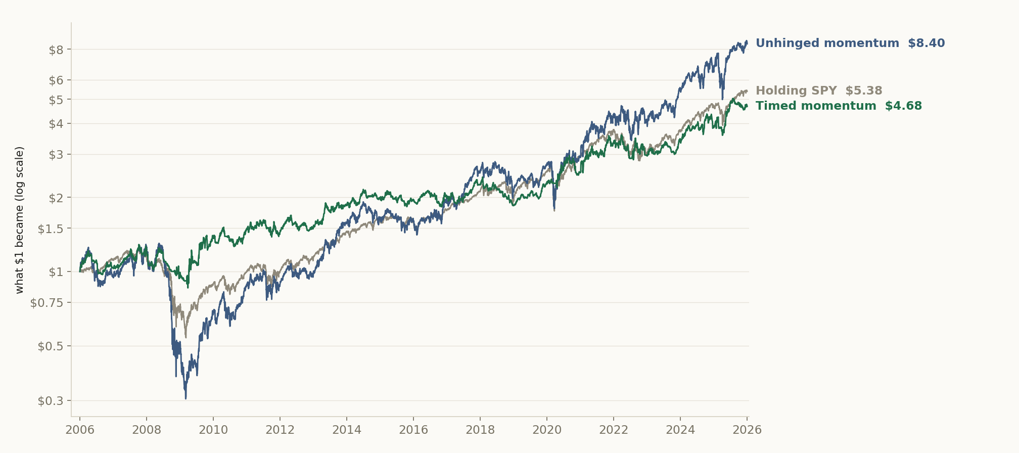
We ran the two portfolios side by side for twenty years, in forty six-month tests, with SPY beside them (Figure 1).

The falls. Unhinged momentum fell 77% from its high in May 2008 to March 2009. SPY fell 56%. Timed momentum fell 33% at worst.

The swings. Measured as volatility, unhinged momentum swung 31% a year, SPY 19% and timed momentum 18%. On the joined daily path, with no cash rate taken off, their Sharpe ratios were 0.50, 0.53 and 0.52: for each unit of risk, neither portfolio did better than SPY. The record further down computes them on the forty tests as recorded and gets 0.47, 0.51 and 0.50.

The growth. $1 became $8.40 with unhinged momentum, $5.38 in SPY and $4.68 with timed momentum: 11.2%, 8.8% and 8.0% a year. Prices leave out dividends in all three. From 2010, timed momentum made far less than SPY.

Part of the calm is cash. On an average day timed momentum had 59% of its money in stocks. We added a yardstick after the tests, its share taken from that result: SPY held at the same share, the rest in cash. It lost 23% in 2008, as much as timed momentum, and swung only 11.5% a year. But it grew 5.6% a year, so timed momentum made 2.4 points a year more, at a higher swing of 18% a year, and its worst fall was smaller, 33% against 37%.

Why. Six of the ten picked in July 2008 were oil, gas, coal and steel stocks, and they fell hard when the commodity boom broke. In 2008 unhinged momentum lost 61%, SPY 38% and timed momentum 23%. The check sells a stock after a few weeks of falling prices, so it was out of most of them early. In rising markets it paid for that. The strongest stocks dip often on the way up, and each dip sent the check out until the price had climbed again. In the 27 six-month tests where the ten rose, timed momentum did better only 3 times. In the 13 where they fell, 9 times.

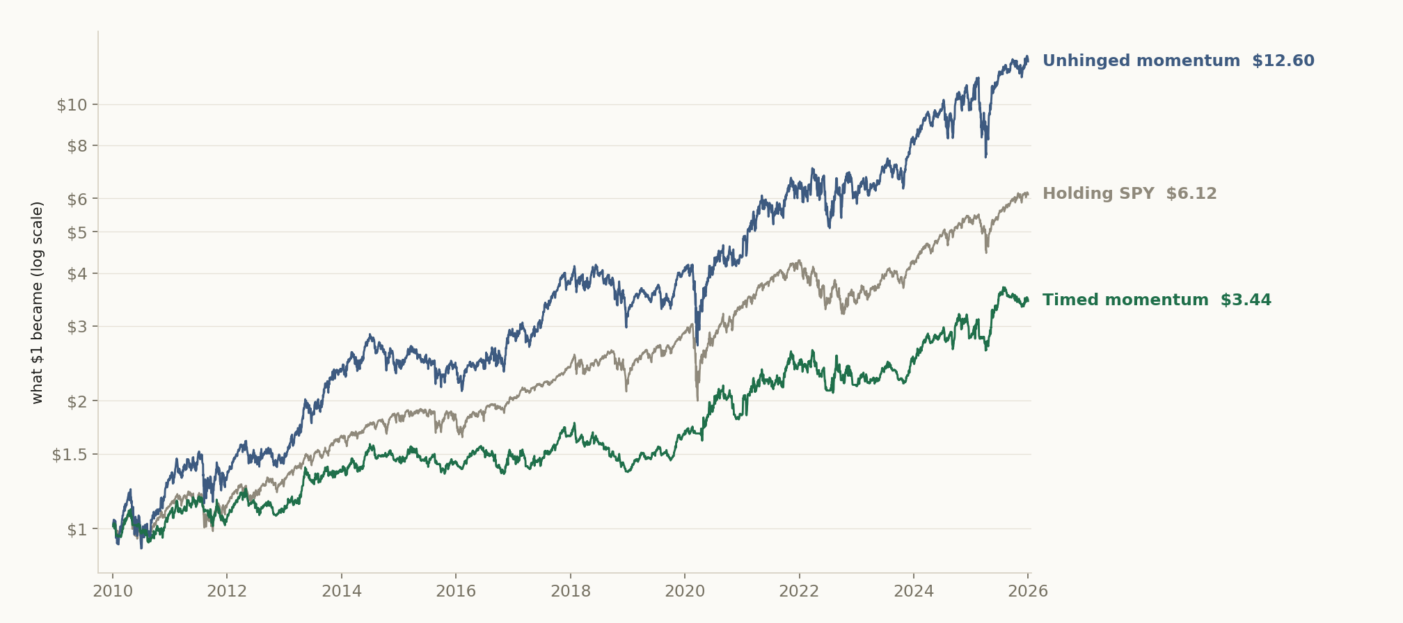
From 2010, after the crash and its rebound, unhinged momentum made 17.2% a year, SPY 12.0% and timed momentum 8.0% (Figure 2). Their worst falls were 36%, 34% and 24%.

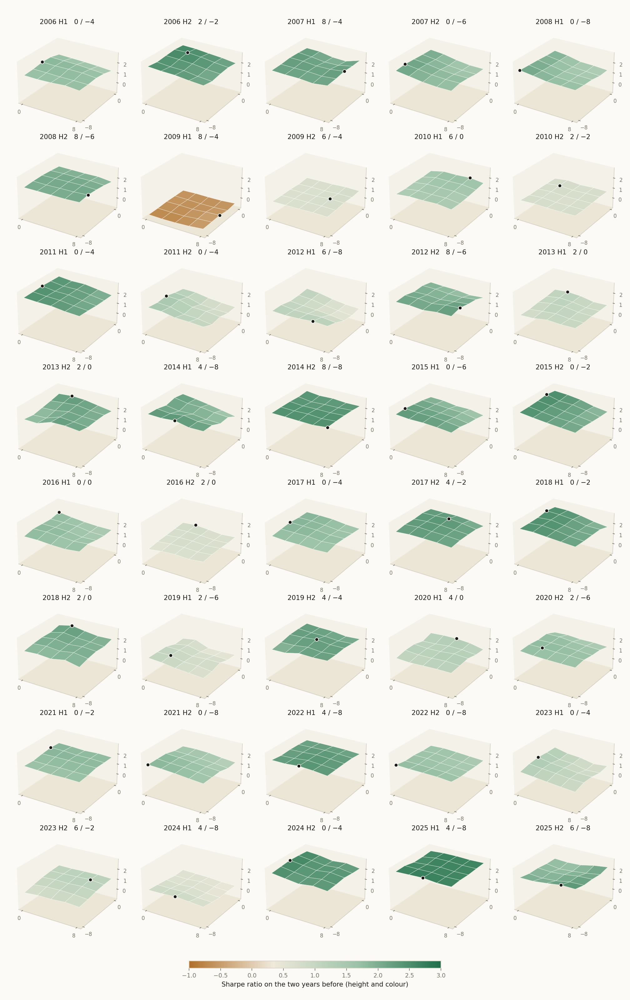
The levels' score on the past was lifted twice (Figure 4). The ten were picked for rising fastest in the same two years, so just holding them there scored a Sharpe ratio of 1.50 on average. The best of the 25 pairs lifted that to 1.89. Measured the same way, test by test, timed momentum then earned 0.57 in the six months after, and unhinged momentum 0.80. The optimizer chose 19 different pairs in the 40 tests, and most of its grids were nearly flat.

**Figure 2.** The same three lines read from the start of 2010, after the 2008 crash and its rebound. Unhinged momentum made 17.2% a year, SPY 12.0% and timed momentum 8.0%.

**Figure 3.** Each six months from 2006 to 2025: timed momentum's return minus unhinged momentum's, in percentage points. Green where the timing added, red where unhinged momentum did better.

**Figure 4.** The optimizer's 40 choices, one small surface for each six-month test. Each surface is the Sharpe ratio the 25 pairs of levels had on the two years before the test. Across is the entry level from 0 to 8%, in depth the exit level from −8 to 0%, and height and colour are the Sharpe ratio. The dark dot is the pair the optimizer chose, given in the title as entry / exit. Most surfaces are nearly flat, and the dot moves from one six months to the next.

1 Methodology, in detail (click to open)

1 Methodology

The stocks. The S&P 500 as its members stood on each first trading day of January and July, 2006 to 2025. Every member with a reliable price history in our data is ranked. The trend is the slope of an ordinary least-squares line through the logarithm of the daily closes over the last 126 trading days, times 252, so it reads as a year's pace. The ten highest slopes are kept. Nothing about the trend is tuned: the 126 days and the ten stocks are fixed before the first test.

The check. The rate of change is 100 times the close divided by the close 20 trading days earlier, minus 100. A buy happens on the day it crosses from below the entry level to above it, a sale on the day it crosses from above the exit level to below it. Timed momentum only buys; it never sells short. The signal is read at the close, and the position is held from that close.

The levels. Before each test, the platform's Static Optimizer runs the 25 pairs of the grid on the same ten stocks over the 730 calendar days before the start, each stock traded with the same pair, a tenth of the money each. It keeps the pair whose equal-weight portfolio had the best Sharpe ratio over those two years. The pair applies to all ten stocks for the next six months and is not changed during them.

The tests. Each six-month test starts in cash. Timed momentum gives each position a fixed tenth of the money, so with ten stocks it can be fully invested but never borrows. Unhinged momentum buys the ten at the first close in equal amounts and does not rebalance. Every trade pays 0.1% of its value, the purchases at the start included. Prices are without dividends in both portfolios and for SPY.

The path. The figures join the 40 tests end to end, from $1 at the first close of 2006 to the last close of 2025. A test that ends on a holiday or a weekend ends at the close before it; the day into the next test's first close is carried with what each portfolio held, as in our recent papers. SPY is the tests' own record of the fund over the same days.

2 Results

Findings

The falls (Figure 1). Unhinged momentum fell 77% from its high in May 2008 to March 2009. SPY fell 56% from October 2007 to March 2009. Timed momentum fell 33% at worst, from October 2007 to March 2009.

The swings. Measured as volatility, unhinged momentum swung 31% a year, SPY 19% and timed momentum 18%. The return for each unit of that risk, the Sharpe ratio on the joined daily path with no cash rate taken off, was 0.50 for unhinged momentum, 0.53 for SPY and 0.52 for timed momentum. Neither portfolio beat SPY on that basis. On the forty tests as recorded, the record further down gets 0.47, 0.51 and 0.50.

Time in stocks. On an average day timed momentum had 59% of its money in stocks. It was fully invested on 10% of the days and all in cash on 3%. Its cash earns no interest in these tests.

SPY with the same cash, a yardstick added after the tests. Held at 59% in stocks and the rest in cash, re-set every day, SPY turned $1 into $2.97, 5.6% a year, and 7.3% a year from 2010. It lost 23% in 2008, fell 37% at worst and swung 11.5% a year. Its Sharpe ratio is SPY's own, 0.53.

The growth. From the first close of 2006 to the last close of 2025, $1 became $8.40 with unhinged momentum, $5.38 in SPY and $4.68 with timed momentum: 11.2%, 8.8% and 8.0% a year. Year by year, unhinged momentum beat SPY in 11 of the 20 years, and timed momentum beat unhinged momentum in 5.

The crash years. In 2008 unhinged momentum lost 61%, SPY 38% and timed momentum 23%. In 2009 timed momentum made 42.6%, unhinged momentum 37.0% and SPY 23.5%. Timed momentum was ahead of unhinged momentum for the last time in September 2020, and ahead of SPY as late as August 2025.

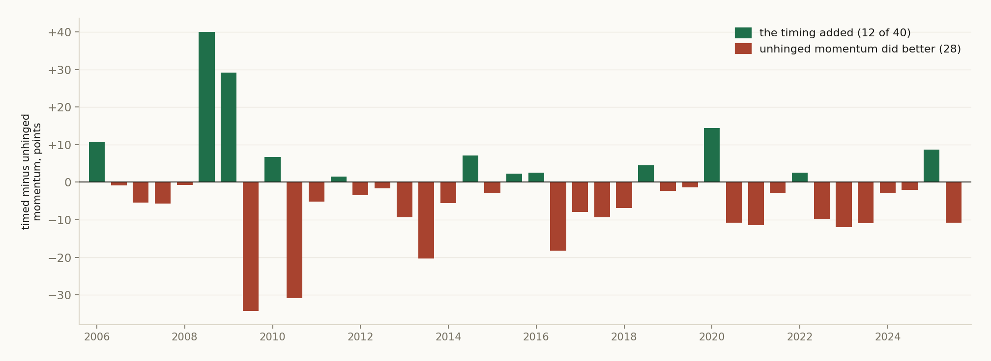
The six-month tests (Figure 3). Timed momentum did better than unhinged momentum in 12 of the 40 tests. In the 13 tests where unhinged momentum lost money, timed momentum did better 9 times. In the 27 where unhinged momentum made money, 3 times.

The costliest years for the timing. In 2013 unhinged momentum made 61.0% and timed momentum 23.5%. In 2010 it was 30.1% against 8.1%, and in 2023 35.6% against 15.6%. Leave out 2008 and 2009, and unhinged momentum made 16.6% a year, SPY 11.5% and timed momentum 8.4%.

The 2010 view (Figure 2). From the last close of 2009, $1 became $12.60 with unhinged momentum, $6.12 in SPY and $3.44 with timed momentum: 17.2%, 12.0% and 8.0% a year. The worst falls from a high were 36%, 34% and 24%. Timed momentum did better than unhinged momentum in 9 of the 32 six-month tests.

The levels (Figure 4, Table 3). The optimizer chose 19 different pairs of levels in the 40 tests. The most common, an entry at 0% and an exit at −4%, was chosen 6 times. In half of the tests, the best pair's Sharpe ratio on the two years before was less than 0.22 above the middle pair of the grid.

The levels' score on the past. On the two years each pair was chosen on, the chosen pairs averaged a Sharpe ratio of 1.89. The ten were picked for rising fastest in that same stretch, and simply holding them there averaged 1.50. So most of the score came from the stocks, and choosing the best of 25 pairs added the rest. Measured the same way, test by test, timed momentum averaged 0.57 in the six months after, and unhinged momentum 0.80. On the past the levels added 0.39 to holding the ten; after, they took 0.23 away.

The stocks (Table 4). NVIDIA was among the ten steepest trends in 11 of the 40 half-years, AMD and Netflix in 7 each, and Freeport-McMoRan in 6. GameStop's four were the first half of 2008, the second half of 2011 and both halves of 2013, years before its 2021 surge.

2.1 Headline

Timed momentum, Sharpe

0.50

day by day, every year the test ran, 2006 to 2025

Unhinged momentum, Sharpe

0.47

day by day, every year the test ran, 2006 to 2025

SPY, Sharpe

0.51

the same days, stitched across the windows

The result

From 2006 to 2025, unhinged momentum on the ten steepest trends turned $1 into $8.40 and fell 77% from its 2008 high. Timed momentum turned $1 into $4.68, and its worst fall was 33%. SPY turned $1 into $5.38 and fell 56%.

Table 1. Each year from 2006 to 2015: its return, prices without dividends; every trade pays 0.1%. Each year runs from the last close of the year before; 2006 starts at its first close.

Year	Unhinged momentum	Timed momentum	SPY
2006	−4.6%	+3.6%	+11.8%
2007	+32.2%	+19.8%	+3.2%
2008	−61.4%	−23.1%	−38.3%
2009	+37.0%	+42.6%	+23.5%
2010	+30.1%	+8.1%	+12.8%
2011	+0.7%	−2.9%	−0.2%
2012	+11.1%	+5.4%	+13.5%
2013	+61.0%	+23.5%	+29.7%
2014	+3.9%	+6.4%	+11.3%
2015	−1.2%	−1.6%	−0.8%

Table 2. Each year from 2016 to 2025: its return, prices without dividends; every trade pays 0.1%. Each year runs from the last close of the year before; 2006 starts at its first close.

Year	Unhinged momentum	Timed momentum	SPY
2016	+17.9%	+2.0%	+9.6%
2017	+32.5%	+13.2%	+19.4%
2018	−14.8%	−17.4%	−6.3%
2019	+26.4%	+22.3%	+28.8%
2020	+7.8%	+11.4%	+16.2%
2021	+47.0%	+30.8%	+27.0%
2022	−4.9%	−10.4%	−19.5%
2023	+35.6%	+15.6%	+24.3%
2024	+16.7%	+11.9%	+23.3%
2025	+30.2%	+22.0%	+16.4%
A year, 2006 to 2025	11.2%	8.0%	8.8%
$1 became	$8.40	$4.68	$5.38

Table 3. How many of the 40 six-month tests traded each pair of levels, the pair with the best Sharpe ratio on the two years before. An empty cell was never chosen.

Entry, rate of change above	exit below 0%	exit below −2%	exit below −4%	exit below −6%	exit below −8%
0%	1	3	6	2	3
2%	4	2		2
4%	1	1	1		4
6%	1	1	1		2
8%			2	2	1

Table 4. How many of the 40 six-month tests had each stock among the ten steepest trends (4 or more).

Ticker	Six-month tests
NVDA	11
AMD	7
NFLX	7
FCX	6
AAPL	5
ALGN	5
AMZN	5
FSLR	5
MRO	5
NRG	5
CNX	4
DVN	4
EA	4
GME	4

Sections 2.2 to 4, the full record: every year, every test, and how each one was run (click to open)

The registration names the two groups compared Timed by the rate of change and The same ten, held; this paper calls them Timed momentum and Unhinged momentum.

2.2 Per-step results

**Table 5.** One row per step, raw out-of-sample results. A short window can pair a negative return with a positive annualised Sharpe: at high daily volatility the arithmetic mean of daily returns sits above the compounded window return, and the Sharpe reads the former. Volatility drag, printed rather than smoothed.
#	Out-of-sample window	Timed momentum SR	Unhinged momentum SR
1	2006-01-03 → 2006-06-30	1.50	0.19
2	2006-07-03 → 2006-12-29	-0.93	-0.41
3	2007-01-03 → 2007-06-29	2.38	1.95
4	2007-07-02 → 2007-12-31	0.65	0.83
5	2008-01-02 → 2008-07-01	-0.14	0.03
6	2008-07-01 → 2008-12-31	-1.98	-1.75
7	2009-01-02 → 2009-07-01	0.65	-0.47
8	2009-07-01 → 2009-12-31	1.77	2.69
9	2010-01-04 → 2010-07-01	-0.46	-0.45
10	2010-07-01 → 2010-12-31	1.35	2.93
11	2011-01-03 → 2011-07-01	1.04	1.26
12	2011-07-01 → 2011-12-30	-1.13	-0.51
13	2012-01-03 → 2012-06-29	1.04	1.16
14	2012-07-02 → 2012-12-31	-0.40	0.01
15	2013-01-02 → 2013-07-01	2.00	2.15
16	2013-07-01 → 2013-12-31	0.68	2.13
17	2014-01-02 → 2014-07-01	2.14	1.98
18	2014-07-01 → 2014-12-31	-1.79	-1.50
19	2015-01-02 → 2015-07-01	-0.09	0.31
20	2015-07-01 → 2015-12-31	-0.06	-0.14
21	2016-01-04 → 2016-07-01	1.67	0.58
22	2016-07-01 → 2016-12-30	-0.39	1.10
23	2017-01-03 → 2017-06-30	-0.05	0.75
24	2017-07-03 → 2017-12-29	2.19	2.46
25	2018-01-02 → 2018-06-29	-0.44	0.41
26	2018-07-02 → 2018-12-31	-2.96	-1.43
27	2019-01-02 → 2019-07-01	2.85	2.34
28	2019-07-01 → 2019-12-31	2.01	1.24
29	2020-01-02 → 2020-07-01	1.27	0.21
30	2020-07-01 → 2020-12-31	-0.26	0.71
31	2021-01-04 → 2021-07-01	1.86	2.12
32	2021-07-01 → 2021-12-31	0.88	0.88
33	2022-01-03 → 2022-07-01	-1.41	-0.77
34	2022-07-01 → 2022-12-30	0.36	0.85
35	2023-01-03 → 2023-06-30	1.91	2.30
36	2023-07-03 → 2023-12-29	0.93	1.49
37	2024-01-02 → 2024-07-01	2.82	2.65
38	2024-07-01 → 2024-12-31	-0.12	0.14
39	2025-01-02 → 2025-07-01	1.98	0.86
40	2025-07-01 → 2025-12-31	-0.36	0.93

Figure 5. Timed momentum: every step's out-of-sample curve overlaid, each rebased to 1× at its own start. Read alongside the per-step table: consistent shape across steps is the walk-forward's evidence; a single lucky leg is not.

Figure 6. Unhinged momentum: the same windows, the other arm. Compare shape-for-shape with the previous figure: the two arms trade the identical out-of-sample windows.

2.3 Search accounting

No search record exists for this design. It was not promoted from a recorded evolving search, so the number of alternatives tried before it, on paper, in another tool, or in the author's head, is unknown. Unknown is a different fact from one: a study with no lineage is not a strategy with one trial, it is a strategy with an unrecorded number of them. Accordingly no count of alternatives tried is claimed, and nothing in this paper is corrected for a search that was never recorded; the number that stands is the raw out-of-sample result plus this disclosure. The registered per-step record below (§4) still guarantees each window's hypothesis was hashed and registered before that window was scored.

2.4 The comparison

Both arms trade the same registered windows, so their returns can be PAIRED: inside each window the two return series are inner-joined date by date and the difference r_{Timed momentum} − r_{Unhinged momentum} is the object under test. Because this is ONE pre-declared contrast, frozen at registration before any window was scored, the paired statistic needs no multiple-testing deflation, and the per-arm pooled numbers above are likewise uncorrected, because this design has no recorded search to correct against (§2.3). The paired contrast carries that gap differently from the arm levels: it was declared before each window ran and it is scored on the difference, so no window could be read first and scored after. What the timestamps cannot speak to is how this contrast came to be the declared one, which is the limit §2.3 states.

In the table: Arm A = Timed momentum · Arm B = Unhinged momentum.

**Table 6.** Window-by-window paired comparison. Δ is the growth gap (Arm A − Arm B) over the window's paired dates.
#	Window	Paired bars	Arm A	Arm B	Δ	Leader
1	2006-01-04 → 2006-06-30	124	+11.3%	+0.7%	+10.6 pp	Arm A
2	2006-07-05 → 2006-12-29	125	-6.4%	-5.4%	-1.0 pp	Arm B
3	2007-01-04 → 2007-06-29	123	+12.3%	+17.8%	-5.5 pp	Arm B
4	2007-07-03 → 2007-12-31	126	+6.3%	+12.1%	-5.7 pp	Arm B
5	2008-01-03 → 2008-07-01	125	-2.5%	-1.6%	-0.9 pp	Arm B
6	2008-07-02 → 2008-12-31	127	-20.3%	-60.3%	+40.0 pp	Arm A
7	2009-01-05 → 2009-07-01	124	+9.7%	-19.3%	+29.0 pp	Arm A
8	2009-07-02 → 2009-12-31	127	+25.0%	+59.4%	-34.4 pp	Arm B
9	2010-01-05 → 2010-07-01	124	-3.8%	-10.4%	+6.6 pp	Arm A
10	2010-07-02 → 2010-12-31	127	+11.0%	+41.9%	-31.0 pp	Arm B
11	2011-01-04 → 2011-07-01	125	+7.6%	+12.9%	-5.3 pp	Arm B
12	2011-07-05 → 2011-12-30	126	-11.3%	-12.8%	+1.4 pp	Arm A
13	2012-01-04 → 2012-06-29	124	+6.3%	+9.8%	-3.5 pp	Arm B
14	2012-07-03 → 2012-12-31	124	-2.5%	-0.8%	-1.7 pp	Arm B
15	2013-01-03 → 2013-07-01	124	+15.8%	+25.3%	-9.5 pp	Arm B
16	2013-07-02 → 2013-12-31	127	+4.8%	+25.2%	-20.4 pp	Arm B
17	2014-01-03 → 2014-07-01	124	+16.2%	+21.8%	-5.6 pp	Arm B
18	2014-07-02 → 2014-12-31	127	-8.1%	-15.2%	+7.1 pp	Arm A
19	2015-01-05 → 2015-07-01	124	-1.1%	+1.9%	-3.0 pp	Arm B
20	2015-07-02 → 2015-12-31	127	-0.6%	-2.8%	+2.2 pp	Arm A
21	2016-01-05 → 2016-07-01	125	+6.8%	+4.3%	+2.5 pp	Arm A
22	2016-07-05 → 2016-12-30	126	-4.0%	+14.4%	-18.3 pp	Arm B
23	2017-01-04 → 2017-06-30	124	-1.2%	+6.9%	-8.0 pp	Arm B
24	2017-07-05 → 2017-12-29	125	+13.3%	+22.7%	-9.5 pp	Arm B
25	2018-01-03 → 2018-06-29	124	-3.4%	+3.5%	-7.0 pp	Arm B
26	2018-07-03 → 2018-12-31	125	-14.1%	-18.6%	+4.5 pp	Arm A
27	2019-01-03 → 2019-07-01	124	+11.6%	+14.0%	-2.4 pp	Arm B
28	2019-07-02 → 2019-12-31	127	+9.5%	+11.1%	-1.5 pp	Arm B
29	2020-01-03 → 2020-07-01	125	+12.8%	-1.6%	+14.4 pp	Arm A
30	2020-07-02 → 2020-12-31	127	-3.2%	+7.7%	-10.9 pp	Arm B
31	2021-01-05 → 2021-07-01	124	+21.2%	+32.7%	-11.6 pp	Arm B
32	2021-07-02 → 2021-12-31	127	+7.9%	+10.9%	-3.0 pp	Arm B
33	2022-01-04 → 2022-07-01	124	-13.9%	-16.4%	+2.5 pp	Arm A
34	2022-07-05 → 2022-12-30	126	+3.0%	+12.8%	-9.8 pp	Arm B
35	2023-01-04 → 2023-06-30	123	+11.1%	+23.1%	-12.1 pp	Arm B
36	2023-07-05 → 2023-12-29	125	+4.7%	+15.7%	-11.0 pp	Arm B
37	2024-01-03 → 2024-07-01	124	+17.7%	+20.7%	-3.0 pp	Arm B
38	2024-07-02 → 2024-12-31	127	-2.5%	-0.4%	-2.1 pp	Arm B
39	2025-01-03 → 2025-07-01	122	+25.0%	+16.4%	+8.6 pp	Arm A
40	2025-07-02 → 2025-12-31	127	-2.7%	+8.1%	-10.8 pp	Arm B

Paired Sharpe of the difference track: -0.28 · block bootstrap (2000 paths, block 10, seed 1234): P(Timed momentum beats Unhinged momentum) = 7.0%.

Window win-rate. Timed momentum led 12 of 40 windows (30.0%), Unhinged momentum led 28, and the mean window gap of -2.98 pp points the same way. Widest single window: 2008 at +40.0 pp.

**Table 7.** The same comparison split at 2010. Pooling the whole walk into one row hides which side of the split the difference came from.
Period	Windows	Timed momentum	Unhinged momentum	Mean gap	Timed momentum led
All windows	40	+4.23%	+7.21%	-2.98 pp	12/40
Before 2010	8	+4.43%	+0.43%	+4.00 pp	3/8
2010 onward	32	+4.18%	+8.90%	-4.72 pp	9/32

Figure 7. Mean window return per period. Timed momentum above, Unhinged momentum below, with the gap at right. The pooled bar and the post-2010 bar are the same comparison over different periods.

The two eras disagree by 8.72 pp. The pooled figure is therefore not a standing property of either method, it is dominated by the later period. Read the two rows, not the average.

3 The circuit

The strategy is a circuit of platform primitives, frozen when the study is registered. Below is the circuit as wired on the canvas, the objective it encodes and how the search runs through it, followed by the mathematics each primitive actually computes, the same formulas the execution engine runs. The complete parameterisation is preserved in the study ledger (Appendix A).

The hypothesis under test

The sentence below is the registered design with its rules in plain words; the exact registration record is in Appendix A2; the authored description of the design is Section 1.

A COMPARATIVE study: Timed by the rate of change vs The same ten, held, walked on the same registered out-of-sample windows. Timed by the rate of change: S&P 500, the highest 10 by Trend slope (126 days), bought when ROC (length 20) crosses above 4; sell when ROC (length 20) crosses below -4, with parameters tuned in-sample to sharpe, and forward-tested out-of-sample from the anchor: the rule set is frozen at the anchor, with no in-sample re-optimization. The same ten, held: S&P 500, the highest 10 by Trend slope (126 days), held as a buy-and-hold basket, and run out-of-sample from the anchor: anything the design estimates from history, where it estimates at all, is re-estimated at each anchor from pre-anchor data only, and the walk advances through registered out-of-sample windows; its disposition is the realized forward path versus the benchmark. The arms differ in: 4 places: Strategy Loader, removed in The same ten, held; Signal Module, removed in The same ten, held; Static Optimizer, removed in The same ten, held; Signal Forward Test → Portfolio Forward Test, substituted (its parameters change with the swap). NOTE: with more than one difference, an out-of-sample gap cannot be attributed to any single change. The contrast under test: whether Timed by the rate of change generates better risk-adjusted returns than The same ten, held over the identical out-of-sample windows.

Every block in this study is a card from the platform's catalog: the S&P 500 as it stood on each day, Trend Slope and Top-N for the ten steepest trends, a Signal Module with the rate-of-change check, the Static Optimizer for its two levels, the Signal Forward Test for timed momentum, the Portfolio Forward Test for unhinged momentum, and a cost of 0.1% on every trade. You can rebuild every test and change any setting.

Figure 8. The frozen circuit, every node a primitive, every wire a typed data-flow; the two arms are colour-coded (Timed momentum green, Unhinged momentum blue, shared feeds neutral). Each box is one step of the strategy; data flows along the wires left to right, and no box can see data dated later than the box feeding it. The whole diagram was frozen when the hypothesis was registered. Click any node to open what that step ran with and what it produced.

Envelopes show counts, ratios, dates, and the parameters the author chose. Full price and per-name data series are not republished: the underlying market data is licensed to QuanterLab. Point figures quoted in the prose, a named holding's return over a stated span, are summary facts derived from public market prices, not redistributed series.

What each part does

Universe, The starting set of tickers, resolved point-in-time from the index change-log, so names delisted or removed later still compete on the dates they traded.

Price Loader, Bulk OHLCV fetch for the whole universe, point-in-time, no future bars.

Filter Trend Slope, Trend slope, the annualized direction and steepness.

Top N, Keep the best N, rank, then cut.

Strategy Loader, Deep-history load for the few names you will actually trade.

Signal Module, The entry / exit rule, turn indicators into a per-bar trade signal.

Static Optimizer, Grid-search one best parameter set over the whole in-sample window.

Backtest Validator, Forward-test the winning rule on unseen, out-of-sample data.

Transaction Cost, Charge for trading, slippage + commission on every turn.

Portfolio Backtest, Replay the portfolio forward, rebalanced, point-in-time, with costs.

The objective and the search

Timed by the rate of change

Universe	S&P 500 index constituents.
Selection	metric across Trend slope (126 days) → highest 10 kept by Trend slope (126 days).
Signal generation	buy when ROC (length 20) crosses above 4; sell when ROC (length 20) crosses below -4.
In-sample search	In-sample optimization via static (single best params across the in-sample); objective = sharpe; sweeping entry.value ∈ [0, 8] / 5 steps × exit.value ∈ [-8, 0] / 5 steps; 252-day in-sample train window.
Validation & out-of-sample	signal forward test (6m horizon from the anchor, each position a fixed 1/10 of the book; a position keeps its size to its exit, new signals take free room, share it equally when it is short, and skip the trade when the book is full); overlays: Transaction Cost.
Other components	Signal: Strategy Loader.

The same ten, held

Validation & out-of-sample	portfolio forward test (holds the weights it is given, re-set at each rebalance) (6m horizon from the anchor, held (no rebalance)); overlays: Transaction Cost.

Every other specification row is identical to Timed by the rate of change's table above.

What differs between the arms, 4 differences; more than one thing changes at once:

removedStrategy Loader, removed in The same ten, held
removedSignal Module, removed in The same ten, held
removedStatic Optimizer, removed in The same ten, held
substitutedSignal Forward Test → Portfolio Forward Test, substituted (its parameters change with the swap)

Reader's note. With 4 settings changed at once across 4 nodes, an out-of-sample gap between the arms cannot be attributed to any single change, the arms are compared as whole packages, and any causal reading of one ingredient is unsupported by this design.

Cost elements are wired into the circuit, the realised drag is reported per step in Appendix B.

Show the mathematics, 10 primitives, formulas and parity notes

3.1 Universe

The starting set of tickers, resolved point-in-time from the index change-log, so names delisted or removed later still compete on the dates they traded.

Before any math, you need a list of stocks. An index preset (S&P 500, Nasdaq-100, Dow 30) is reconstructed as it stood ON your anchor date by replaying the historical add/drop change-log backwards, so a 2018 backtest sees the 2018 membership, not today's winners.

Point-in-time membership

Start from today's constituents and un-apply every membership change after the anchor t:

\mathcal{U}(t) = \mathcal{U}_{\text{now}} \;\ominus\; \{\text{adds after } t\} \;\oplus\; \{\text{drops after } t\}

Constituents resolved from the index change-log; the same point-in-time set the factor + screening modules use.

3.2 Price Loader

Bulk OHLCV fetch for the whole universe, point-in-time, no future bars.

Momentum, volatility, trend, every price-based metric needs history. This loads open/high/low/close/volume for all names in parallel, clipped so nothing after the anchor can leak in. The lookback window is derived automatically from the deepest metric you wired.

The window is derived, not guessed

It loads exactly enough history for the hungriest downstream metric plus a warm-up buffer:

W = \max_k(\text{lookback}_k) + \text{buffer}, \qquad \text{bars} \le \text{anchor } t

3.3 Filter Trend Slope

Trend slope, the annualized direction and steepness.

The slope of a straight line fitted to log-price, scaled to a yearly rate. Signed: strongly positive is a powerful uptrend, negative a downtrend. The line is fitted over about six months unless you set the window. With "Steadiness counts" on, it is the ranking of Andreas Clenow's Stocks on the Move: the yearly speed times how straight the line is, so a steady climb ranks above a jumpy one of the same speed.

Annualized OLS slope

\text{slope}_{\text{ann}} = b \times 252, \qquad \log P_\tau = a + b\,\tau

Fitted over the last n trading days: 126 unless set (Clenow uses 90).

With "Steadiness counts" (Clenow)

\text{score} = \left(e^{\,252\,b} - 1\right) \times R^2

The slope compounded over a year, times the R² of the same fit. A line that explains the prices well keeps most of its speed; a choppy one loses it.

3.4 Top N

Keep the best N, rank, then cut.

Sort the survivors by the Composite Σ (or, if none is wired, the last metric in the chain) and keep the top (or bottom) N. The final narrowing from a scored list to a committed basket.

Order statistic cut

\text{Top-}N = \{\, i : \operatorname{rank}(\text{score}_i) \le N \,\}

"Keep highest" for momentum; "keep lowest" for e.g. Hurst (mean reversion).

Or a share of the ranked names

N = \operatorname{round}(f \cdot n_{\text{ranked}})

With a fraction f above 0 (0.3333 is a third), N follows the number of names that have a value at the anchor, so a third stays a third when fewer names are priced. A skip fraction takes a share off the end first: 0.3333 with skip 0.3333 is the middle third.

Keep what you hold (when set)

\text{kept} = \{\, i \in H : \operatorname{rank}_i \le K \,\} \;\cup\; \text{best ranked } i \notin H \text{ up to } N

In a Portfolio Forward Test that re-selects, H is what the book holds. A held name stays while it ranks within K places; the free places go to the best ranked names. Clenow keeps a stock while it is in the top 20% of the S&P 500, about K = 100. Unset, K is 0 and the top N are taken fresh.

3.5 Transaction Cost

Charge for trading, slippage + commission on every turn.

Real trading isn't free. This deducts a cost proportional to how much you trade (turnover), in basis points, so the backtest reflects net, not gross, performance.

Cost per rebalance

\text{cost}_t = \frac{\text{bps}}{10{,}000}\;\times\;\text{turnover}_t, \qquad \text{turnover}_t = \tfrac12\sum_i \lvert w_{i,t}-w_{i,t^-}\rvert

3.6 Strategy Loader

Deep-history load for the few names you will actually trade.

The efficiency split: screening scans ~1 year across ~500 names, but the lifecycle (signal → optimizer → walk-forward) needs years of history. So this loads that deep window ONLY for the handful of survivors. No new math, the window is derived from the deepest lifecycle lookback (default ~5 years).

Derived deep window, survivors only

W_{\text{deep}} = \max(\text{lifecycle lookbacks}) \approx 5\text{y}, \quad \text{loaded for } \mathcal{S} \text{ only}

3.7 Signal Module

The entry / exit rule, turn indicators into a per-bar trade signal.

Composes indicators (RSI, moving averages, …) with comparison and logic operators into a rule that says enter, exit, or hold each bar. The rule is emitted as a portable config the optimizer tunes and the walk-forward validates, so what you design is exactly what gets traded.

Boolean rule → position state

\text{signal}_t = \begin{cases} +1 & \text{entry rule true} \\ 0 & \text{exit rule true} \\ \text{hold} & \text{otherwise}\end{cases}

e.g. enter when RSI < 30, exit when RSI > 50.

3.8 Static Optimizer

Grid-search one best parameter set over the whole in-sample window.

Sweeps a grid of parameter combinations, backtests each on the in-sample data, and keeps the single combination that scores best on your objective (Sharpe by default). One rule for the whole period, no time variation.

Argmax over the grid

\boldsymbol\theta^* = \arg\max_{\boldsymbol\theta\in\text{grid}} \;\mathcal O\big(\text{backtest}(\boldsymbol\theta)\big)

Objective 𝒪 ∈ {Sharpe, Calmar, Sortino, total return, profit factor, win rate}.

Default objective, Sharpe

\text{Sharpe} = \frac{\bar r - r_f}{\sigma_r}\,\sqrt{252}

3.9 Backtest Validator

Forward-test the winning rule on unseen, out-of-sample data.

Takes the wired rule config (the Walk-Forward validated config wins, else the optimized config, else the raw signal config) and trades it FORWARD on the out-of-sample window to the right of the anchor, data it never saw during optimization, re-deriving the regime as-of each bar. It produces the true out-of-sample equity curve, trades and statistics: the signal-path twin of the Portfolio Forward Test, not an in-sample replay.

Apply the frozen rule forward (OOS)

E_t = E_{t-1}\,(1 + r_t),\qquad \text{Sharpe} = \frac{\bar r - r_f}{\sigma_r}\sqrt{252}

Config frozen from optimization / walk-forward, then replayed bar-by-bar on the forward window it has never seen, with cost + risk overlays applied.

3.10 Portfolio Backtest

Replay the portfolio forward, rebalanced, point-in-time, with costs.

Holds the basket and rebalances on schedule, re-selecting and re-optimizing point-in-time at each rebalance (so it only ever uses information available then), and reports the equity curve, Sharpe, drawdown and trade stats, optionally net of cost and risk overlays.

Compounded equity

E_t = E_{t-1}\big(1 + \mathbf w_{t}^{\top}\mathbf r_t - \text{costs}_t\big)

Drawdown

\text{DD}_t = \frac{E_t}{\max_{\tau\le t}E_\tau} - 1, \qquad \text{MaxDD} = \min_t \text{DD}_t

Financing a levered book

\text{charge}_t \;=\; \text{loan}_t \cdot \frac{\text{spread}}{252}, \qquad \text{loan}_t = \begin{cases}\max(0,\,-\text{cash}_t) & \text{institutional (netted)}\\ \max(0,\,\text{long MV}_t - E_t) & \text{retail (no netting)}\end{cases}

A levered long/short book (the β-neutral Long/Short Select) borrows its excess notional. WHO you are decides the loan: a prime broker nets short-sale proceeds against the margin loan, a fully-netted BAB book carries almost none, while a retail margin account cannot net, so the same book borrows the long leg’s excess over equity. Profiles: institutional = 50 bps spread + 25 bps GC short borrow; retail = 350 bps + 150 bps (the BEST retail tier, so any verdict is conservative); custom = your own knobs, spread on negative cash. Charged daily, reported as financing_drag_pct, never silent.

When the regime only decides the buys

\mathbf w_k = \{\, w_{k,i} : i \in \text{held} \,\}, \qquad \text{cash}_k = 1 - \textstyle\sum_{i \in \text{held}} w_{k,i}

Set "The regime decides" to "Only whether new names are bought": at a rebalance whose regime has an exposure of 0, the new selection keeps only the names already held, each at its weight in the new book; a name that left is sold and its money waits in cash until a rebalance in a regime that buys. Nothing is scaled day to day. Clenow buys only while the S&P 500 is above its 200-day average.

4 Projection calibration, pooled across the walk

Every rebalance carried a Monte Carlo cone and a 95% VaR estimated before the segment it is scored against. Two questions, pooled over the whole study: did realized outcomes land inside the band as often as the band claims, and were VaR breaches as frequent as 5%?

This section is produced by the forward tester itself: every portfolio backtest fits the cone and the VaR estimate at each rebalance and scores them against the segment that followed. It does not require, and this circuit does not contain, a Monte Carlo primitive; that primitive is a separate, standalone analysis.

Figure 9. Projected range versus what occurred, at each of 40 scored rebalance segments. The final rebalance of each step has no following segment to score, the ledger marks those rows “no segment follows this rebalance”, which is why this count sits below the raw rebalance totals in the table beneath. Each vertical bar is that rebalance's P5–P95 Monte Carlo cone with the median ticked; the dot is the realized return of the segment that followed. Filled green = the outcome landed inside its own cone; red = it did not. The strip beneath repeats that as one mark per rebalance, so a run of misses in one period is visible as a run. Every cone was fitted only on data prior to the segment it is scored against.

Arm	Steps	Rebalances	In band	Coverage	Expected	VaR days	Breach rate	Expected
Unhinged momentum	40	40	34 / 40	85.0% ±5.65	90.0%	5005	7.05% ±0.362	5.0%

± values are binomial standard errors on the estimate. A coverage figure below the expected band means the projection was over-confident; a breach rate above 5% means the same of the risk model. Both forecasts used only data prior to the segment scored.

5 Discussion

5.1 Interpretation

We expected the check to cost some growth. We did not expect it to change the portfolio this much. Unhinged momentum on the ten steepest trends swung like a single risky stock, and in 2008 it lost 61%. The same stocks, timed, swung a little less than SPY and lost 23% that year. Part of that calm is cash: timed momentum was in stocks 59% of the time, and SPY held at that share lost about the same in 2008. What the timing added over such a mix was growth, 2.4 points a year, at a higher swing: 18% a year against 11.5%.

The mechanism is plain. After a few weeks of falling prices the 20-day rate of change drops below the exit level, so the check is out of a stock before most of a long fall. The same mechanism costs in the rises. The steepest trends often dip on the way up. Each dip sends the check out, and it buys back only after the price has climbed again, paying 0.1% each way. In the 27 six-month tests where the ten rose, timed momentum came out ahead only 3 times.

Choosing the levels on the past added little. The ten were picked for rising fastest in the same two years the levels were chosen on, so any levels looked good there: holding the ten scored 1.50, the best pair 1.89. Most grids were nearly flat, so the best pair won by a hair and changed from one six months to the next: 19 different pairs in 40 tests. This is the gap the deflated Sharpe ratio warns about, made larger by the way the stocks were picked.

We saw the same shape in our paper on Clenow's Stocks on the Move. There a market switch kept the book's portfolio out of the 2008 crash and cost it in the rising years after. Here the rate-of-change check did that job for each stock on its own.

So the two portfolios are two characters, and which one is better depends on the trader. Unhinged momentum grew 2.4 points a year faster than SPY, and 5.2 faster from 2010, and fell 77% on the way. Timed momentum kept most of the market's gain over the twenty years, though far less of it from 2010, fell 33% at worst, and was in stocks a little over half of the time.

5.2 Limitations

Forty six-month tests are not many, and one crash shapes the result. Without 2008 and 2009 timed momentum trails both others by far more.

Prices only. All three lines leave dividends out, because the test that runs the rate-of-change check counts prices only. SPY paid about 2% a year over these twenty years, probably more than the trend leaders. With dividends, unhinged momentum's lead over SPY would be smaller and timed momentum's gap to SPY larger.

No interest on cash. Timed momentum's cash earns nothing in these tests. With interest on its cash it would have made somewhat more, and so would SPY held with the same cash.

Our price data has no prices for many companies that later left the S&P 500: about a third of the index in 2006, under a tenth from 2015. Such a company can never be among the ten. This probably flatters both portfolios against SPY, whose record is complete, and unhinged momentum more, because it never sells.

The check has many settings and we tried one of each: a 20-day rate of change, one grid of 25 pairs, two years of past to choose on, and the Sharpe ratio to choose by. The ten are chosen again every six months, the shortest test the platform runs for a timed rule. Other choices would give other results.

An earlier run of the same tests, written down and locked at 15:40 UTC on 21 October 2026, started in 2010 by mistake. All our stock studies start in 2006, so we locked a new run from there at 16:12 UTC. That first run pointed the other way: from 2010 to 2025 timed momentum made 8.0% a year against SPY's 12.0%, and its only advantage was smaller falls. Its 32 six-month tests are the last 32 here, unchanged, and Figure 2 shows that stretch.

Try it yourself

Every test in this paper can be run again on quanterlab.com, and you can change any setting. Open it in the lab and try, for example:

• another filter to pick the stocks, such as twelve-month momentum, closeness to the 52-week high, or Clenow's steady trend (the slope times how straight the line is);

• another optimisation: a wider grid, another score than the Sharpe ratio, or levels that change with the market's mood;

• 20 stocks in the pool instead of 10;

• a shorter or a longer rate of change than 20 days.

Or ask the lab assistant to build a version for you, in your own words, and watch it build the test step by step. On Practitioner and Research, a version you like can start live on paper, with a note on it every morning.

References

Author’s references?

QuanterLab (2026). Clenow's Stocks on the Move, tested apart ten years after the book. The steady-trend ranking this paper's ranking comes from, with its market switch. https://quanterlab.com/research/clenow-s-stocks-on-the-move-tested-apart-ten-years-after-the-book
Clenow, A. F. (2015). Stocks on the Move: Beating the Market with Hedge Fund Momentum Strategies. Ranks stocks by the slope of their trend line, there multiplied by how straight the line is.
Jegadeesh, N. and Titman, S. (1993). Returns to buying winners and selling losers: Implications for stock market efficiency. Journal of Finance 48(1), 65-91. https://doi.org/10.1111/j.1540-6261.1993.tb04702.x
Moskowitz, T. J., Ooi, Y. H. and Pedersen, L. H. (2012). Time series momentum. Journal of Financial Economics 104(2), 228-250. A trend measured on each asset's own past, the kind of signal the rate of change is. https://doi.org/10.1016/j.jfineco.2011.11.003
Murphy, J. J. (1999). Technical Analysis of the Financial Markets. New York Institute of Finance. The rate of change among the momentum oscillators.
Pardo, R. (2008). The Evaluation and Optimization of Trading Strategies, 2nd edition. Wiley. Choosing a rule's settings on the past and testing them on the period after, again and again.
Bailey, D. H. and López de Prado, M. (2014). The deflated Sharpe ratio: Correcting for selection bias, backtest overfitting and non-normality. Journal of Portfolio Management 40(5), 94-107. Why the best of many settings looks better on the past than it will after.

Appendix A Reproducibility in QuanterLab

Each step is backed by a frozen run report. The study is re-derivable from the ledger below.

#	Commit	Report	Anchor	OOS window
1	6151f08d71a9	14951	2006-01-01	2006-01-03 → 2006-06-30
2	3811326d8c1c	14952	2006-07-01	2006-07-03 → 2006-12-29
3	6075ab531121	14953	2007-01-01	2007-01-03 → 2007-06-29
4	a73b5f068fff	14954	2007-07-01	2007-07-02 → 2007-12-31
5	f3a2fadf1006	14955	2008-01-01	2008-01-02 → 2008-07-01
6	f9e6b8a357bd	14956	2008-07-01	2008-07-01 → 2008-12-31
7	9d542e670201	14957	2009-01-01	2009-01-02 → 2009-07-01
8	510b6554220c	14958	2009-07-01	2009-07-01 → 2009-12-31
9	213aabe763a1	14959	2010-01-01	2010-01-04 → 2010-07-01
10	6bca08e7669e	14960	2010-07-01	2010-07-01 → 2010-12-31
11	59b4afbb6867	14961	2011-01-01	2011-01-03 → 2011-07-01
12	f5420c47ec59	14962	2011-07-01	2011-07-01 → 2011-12-30
13	17bd611d91e7	14963	2012-01-01	2012-01-03 → 2012-06-29
14	aa4a8c523964	14964	2012-07-01	2012-07-02 → 2012-12-31
15	d299ac1ba9d1	14965	2013-01-01	2013-01-02 → 2013-07-01
16	0610834e2e7c	14966	2013-07-01	2013-07-01 → 2013-12-31
17	faf51f941e13	14967	2014-01-01	2014-01-02 → 2014-07-01
18	c01e289884bc	14968	2014-07-01	2014-07-01 → 2014-12-31
19	6caaee1831c7	14969	2015-01-01	2015-01-02 → 2015-07-01
20	aaa9f8465e29	14970	2015-07-01	2015-07-01 → 2015-12-31
21	bcf863c51055	14971	2016-01-01	2016-01-04 → 2016-07-01
22	03bea9d7e7ed	14972	2016-07-01	2016-07-01 → 2016-12-30
23	0600fb7f4748	14973	2017-01-01	2017-01-03 → 2017-06-30
24	d96afcc95753	14974	2017-07-01	2017-07-03 → 2017-12-29
25	3323942098f9	14975	2018-01-01	2018-01-02 → 2018-06-29
26	215c8b271304	14976	2018-07-01	2018-07-02 → 2018-12-31
27	6deab757c4f5	14977	2019-01-01	2019-01-02 → 2019-07-01
28	3c353a20a3b0	14978	2019-07-01	2019-07-01 → 2019-12-31
29	6bbe3717bfc4	14979	2020-01-01	2020-01-02 → 2020-07-01
30	d5b0a7db0181	14980	2020-07-01	2020-07-01 → 2020-12-31
31	c535c8b06340	14981	2021-01-01	2021-01-04 → 2021-07-01
32	ff2ff4bd7570	14982	2021-07-01	2021-07-01 → 2021-12-31
33	ce56249815b3	14983	2022-01-01	2022-01-03 → 2022-07-01
34	4b08adf450b1	14984	2022-07-01	2022-07-01 → 2022-12-30
35	08bcad08cbd5	14985	2023-01-01	2023-01-03 → 2023-06-30
36	84d7d1914146	14986	2023-07-01	2023-07-03 → 2023-12-29
37	c84175f32c77	14987	2024-01-01	2024-01-02 → 2024-07-01
38	999cfb3052ed	14988	2024-07-01	2024-07-01 → 2024-12-31
39	5309702a406a	14989	2025-01-01	2025-01-02 → 2025-07-01
40	4abbeee59afc	14990	2025-07-01	2025-07-01 → 2025-12-31

QuanterLab reference architecture

The methods the platform implements, for every study made on it, rest on these works.

Gelman, A., & Loken, E. (2013). The garden of forking paths: Why multiple comparisons can be a problem, even when there is no “fishing expedition.” Working paper, Columbia University.
Harvey, C. R., Liu, Y., & Zhu, H. (2016). … and the Cross-Section of Expected Returns. Review of Financial Studies, 29(1), 5–68. doi:10.1093/rfs/hhv059
Lo, A. W. (2002). The Statistics of Sharpe Ratios. Financial Analysts Journal, 58(4), 36–52. doi:10.2469/faj.v58.n4.2453

Appendix A2 Registration record

What this record does and does not establish. Every window in this study is historical: the data existed before the study began, so this is sequential registration on past windows, not pre-registration in the clinical-trial sense, and no procedure could make it so. What the platform does enforce is order, each step's specification was frozen and hashed before that step was scored, and the walk cannot advance past a step that was never run or close one with a result registered for a different window. The two timestamp columns below are the evidence: read them together and each registration precedes its own run, and each run precedes the next registration. A study whose registrations all post-date its runs would show it here. Wall-clock spacing between registrations varies with the author's schedule and queue latency; the ordering, not the tempo, is the claim.

“A COMPARATIVE study: Timed by the rate of change vs The same ten, held, walked on the same registered out-of-sample windows. Timed by the rate of change: S&P 500, the highest 10 by Trend slope (126 days), bought when ROC (length 20) crosses above 4; sell when ROC (length 20) crosses below -4, with parameters tuned in-sample to sharpe, and forward-tested out-of-sample from the anchor: the rule set is frozen at the anchor, with no in-sample re-optimization. The same ten, held: S&P 500, the highest 10 by Trend slope (126 days), held as a buy-and-hold basket, and run out-of-sample from the anchor: anything the design estimates from history, where it estimates at all, is re-estimated at each anchor from pre-anchor data only, and the walk advances through registered out-of-sample windows; its disposition is the realized forward path versus the benchmark. The arms differ in: 4 places: Strategy Loader, removed in The same ten, held; Signal Module, removed in The same ten, held; Static Optimizer, removed in The same ten, held; Signal Forward Test → Portfolio Forward Test, substituted (its parameters change with the swap). NOTE: with more than one difference, an out-of-sample gap cannot be attributed to any single change. The contrast under test: whether Timed by the rate of change generates better risk-adjusted returns than The same ten, held over the identical out-of-sample windows.”

The same hypothesis was registered independently at every step, hashed before each step's out-of-sample window was scored:

**Table 8.** Registration audit, one row per registered step, with the time each specification was frozen and the time its window was scored. The hypothesis is identical on every row by design: it was registered once and re-registered unchanged at each anchor. Rows that differ would mean the specification moved mid-walk, which is the thing this record exists to rule out. The timestamps are the separate claim: each registration precedes its own run, and each run precedes the next registration.
#	Anchor	Registered at (UTC)	Run completed (UTC)
1	2006-01-01	2026-10-21 16:12:13	2026-10-21 16:12:25
2	2006-07-01	2026-10-21 16:12:25	2026-10-21 16:12:37
3	2007-01-01	2026-10-21 16:12:37	2026-10-21 16:12:50
4	2007-07-01	2026-10-21 16:12:50	2026-10-21 16:13:02
5	2008-01-01	2026-10-21 16:13:02	2026-10-21 16:13:14
6	2008-07-01	2026-10-21 16:13:14	2026-10-21 16:13:39
7	2009-01-01	2026-10-21 16:13:39	2026-10-21 16:14:03
8	2009-07-01	2026-10-21 16:14:03	2026-10-21 16:14:15
9	2010-01-01	2026-10-21 16:14:15	2026-10-21 16:14:28
10	2010-07-01	2026-10-21 16:14:28	2026-10-21 16:14:40
11	2011-01-01	2026-10-21 16:14:40	2026-10-21 16:14:52
12	2011-07-01	2026-10-21 16:14:52	2026-10-21 16:15:05
13	2012-01-01	2026-10-21 16:15:05	2026-10-21 16:15:17
14	2012-07-01	2026-10-21 16:15:17	2026-10-21 16:15:29
15	2013-01-01	2026-10-21 16:15:29	2026-10-21 16:15:42
16	2013-07-01	2026-10-21 16:15:42	2026-10-21 16:15:54
17	2014-01-01	2026-10-21 16:15:54	2026-10-21 16:16:06
18	2014-07-01	2026-10-21 16:16:06	2026-10-21 16:16:18
19	2015-01-01	2026-10-21 16:16:19	2026-10-21 16:16:31
20	2015-07-01	2026-10-21 16:16:31	2026-10-21 16:16:43
21	2016-01-01	2026-10-21 16:16:43	2026-10-21 16:16:55
22	2016-07-01	2026-10-21 16:16:56	2026-10-21 16:17:08
23	2017-01-01	2026-10-21 16:17:08	2026-10-21 16:17:20
24	2017-07-01	2026-10-21 16:17:20	2026-10-21 16:17:32
25	2018-01-01	2026-10-21 16:17:33	2026-10-21 16:17:45
26	2018-07-01	2026-10-21 16:17:45	2026-10-21 16:17:57
27	2019-01-01	2026-10-21 16:17:57	2026-10-21 16:18:22
28	2019-07-01	2026-10-21 16:18:23	2026-10-21 16:18:35
29	2020-01-01	2026-10-21 16:18:35	2026-10-21 16:18:47
30	2020-07-01	2026-10-21 16:18:47	2026-10-21 16:18:59
31	2021-01-01	2026-10-21 16:19:00	2026-10-21 16:19:12
32	2021-07-01	2026-10-21 16:19:12	2026-10-21 16:19:24
33	2022-01-01	2026-10-21 16:19:24	2026-10-21 16:19:36
34	2022-07-01	2026-10-21 16:19:37	2026-10-21 16:19:49
35	2023-01-01	2026-10-21 16:19:49	2026-10-21 16:20:01
36	2023-07-01	2026-10-21 16:20:01	2026-10-21 16:20:14
37	2024-01-01	2026-10-21 16:20:14	2026-10-21 16:20:26
38	2024-07-01	2026-10-21 16:20:26	2026-10-21 16:20:38
39	2025-01-01	2026-10-21 16:20:38	2026-10-21 16:20:51
40	2025-07-01	2026-10-21 16:20:51	2026-10-21 16:21:03

Appendix B Per-step diagnostics

Realized in the projection tables below is the risk engine scoring its own forecast: the buy-and-hold return of the segment that followed each rebalance, on the same gross basis the cone was projected on. It is deliberately not the charged, calendar-window total return the study’s tables print, so the two will not reconcile line by line; the cone and its outcome share one basis, which is what a calibration test requires. Each row names its segment’s span so a boundary session is visible.

Names held is the union across the window: the count of distinct instruments the book touched between the window’s first and last session, not the number it held at one time. A book that rotates monthly touches more names than it holds.

What each step's run actually did beyond its return: the portfolio book's rebalancing and cost drag, and how positions were sized. Harvested from the frozen run reports, present where the circuit produced them. Cost drag is the gap between the step's return before and after its trading costs, in percentage points of the step's starting capital, so on a book that trades every session and compounds it can exceed the step's own net return.

Open the full per-step grid (40 steps: every rebalance and sizing, per window)

Step 1 · 2006-01-03 → 2006-06-30

Unhinged momentum

Portfolio book, rebalanced none · 1 constructions · 10 names held · selection: hold · 0.0% in cash · turnover 1.0× · cost drag 0.1%

Projection accuracy, realized outcome fell inside the P5–P95 cone in 100.0% of 1 scored rebalances (a well-calibrated 90% band contains ~90.0%) · 95% VaR breached on 7.26% of 124 days (expected ~5.0%)

Rebalance	P5	Median	P95	Realized	In band	VaR 95 (1d)	Breaches
2006-01-01 → window end	-12.1137%	14.7817%	50.1173%	1.4685%	yes	2.2341%	9 / 124