


Ornstein-Uhlenbeck Mean Reversion Process Applied on S&P 500 Point-in-Time Constituents over 20 Years: Short Half-Life Against Trending Assets
The Ornstein-Uhlenbeck process is the textbook model of mean reversion: a price that wanders away from its usual level is pulled back toward it, like a ball on a spring. Traders use it to buy a stock when its price is unusually far below its estimated level, and to sell when the price has come back. One number in the model matters most for a trader: the half-life, how many days a gap between the price and its level takes to shrink by half. A short half-life means a strong, quick pull. A trending stock has almost none.
We tested whether the half-life tells a trader where to use the model. Every six months for twenty years we measured the half-life of every stock in the S&P 500 with a price history in our data, as the index stood on that date. One portfolio took the five stocks with the shortest half-life. The other took five trending stocks, with long half-lives and rising prices. Both traded their stocks with the same Ornstein-Uhlenbeck rule, using the buy and sell lines of the best-known practitioners' study of it: the same settings for every stock, fixed in advance, none of them fitted to past results. We sized the trades three ways, including the Kelly formula, and compared the results with SPY, the fund that follows the S&P 500, both as they ran and at the same level of risk.
The rule did better on the short half-life stocks than on the trending stocks, with every way of sizing the trades, and it fell less in the financial crisis. Its trades on the short half-life stocks won more often. Because the rule waits in cash between trades, it made less money than SPY as it ran. Held at the same level of risk as SPY, the short half-life portfolio ended ahead of it before trading costs. The test cannot say how much of the difference between the two groups comes from the half-life itself and how much from avoiding trending stocks. The Kelly formula changed little.
What the Ornstein-Uhlenbeck process is
The Ornstein-Uhlenbeck process is a mathematical model of something that moves randomly but is always pulled back toward a resting level. Two physicists, Leonard Ornstein and George Uhlenbeck, described it in 1930 for the speed of tiny particles moving in a liquid, which friction keeps pulling back toward zero. In finance it became the standard model of mean reversion: a price, or the gap between two prices, that drifts away from its usual level and is pulled back again.
The model has three parts:
• the level the price is pulled toward, called the mean;
• how strong the pull is. The easiest way to read it is the half-life: the number of trading days it takes for a gap between the price and the mean to shrink by half. With a half-life of five days, a price that is ten dollars above its mean is expected to be about five dollars above it a week later;
• how large the random pushes are, which sets how far the price usually is from its mean, its usual spread.
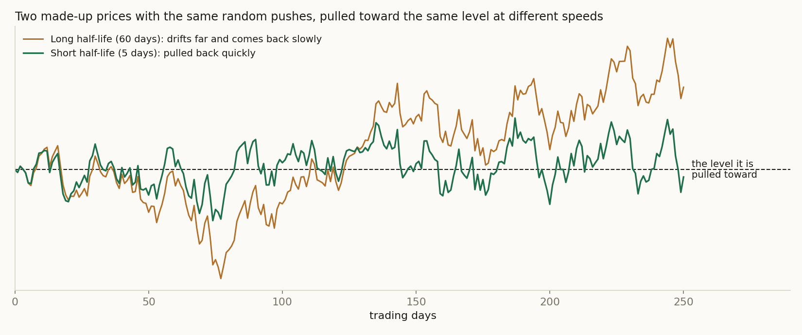
Figure 1 shows two made-up prices with the same random pushes and the same mean. The one with a half-life of 5 days stays close to the mean and keeps coming back. The one with a half-life of 60 days wanders far away and returns slowly. Over a few months it looks like a trend.
How traders use it. Every day, a trader estimates the mean and the usual spread from recent prices and measures how far today's price is from the mean, counted in usual spreads. This count is the z-score. A z-score of −1.25 means the price is 1.25 usual spreads below the mean. The rule buys when the z-score is low, expecting the pull back toward the mean, and sells when the price has come back.
The rule works only where the pull is real. A stock with a short half-life gives it many trips back to the mean. A trending stock has little pull: its price keeps moving away, and the rule buys too early. So the half-life is a natural way to choose where to use the rule. That is what this study tests.
The rule on two real stocks
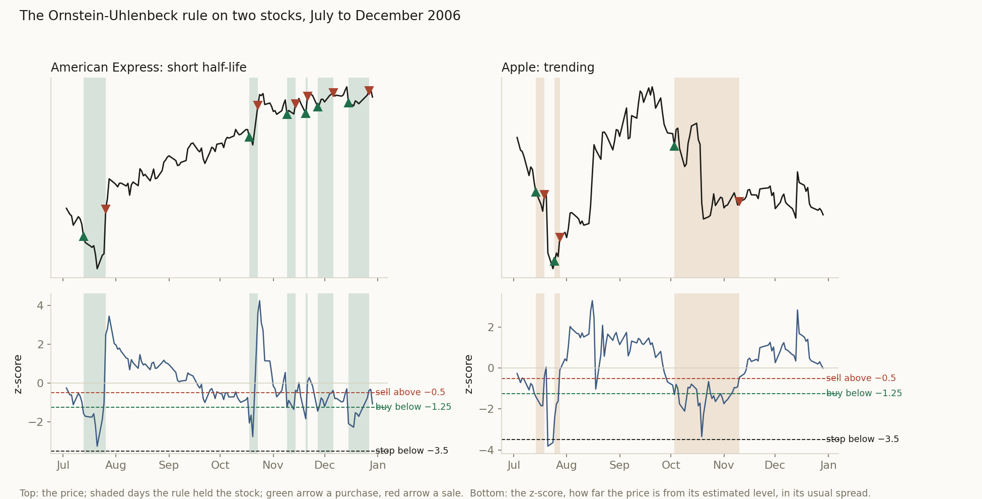
Figure 2 shows the same rule on two stocks in the second half of 2006.
American Express was among the five stocks with the shortest half-life in the year before, about six trading days. The rule bought it six times, each time when its z-score fell below −1.25, and sold each time with a gain when the z-score came back above −0.5.
Apple was among the trending stocks: in the year before, its price had risen and showed no measurable pull back at all. The rule bought Apple three times. One trade made money quickly. The last one, in early October, bought into a fall that kept going, and the rule sold at a loss in November.
The rules, step by step
Both portfolios trade the same rule. Only step 2 differs between them.
Every six months, on the first trading day of January and of July:
1. Take the stocks. All members of the S&P 500 on that day that have a price history in our data, as the index stood then, not as it stands today.
2. Measure each stock's half-life and pick five. For each stock, take the past year of prices, remove its straight-line trend, and estimate how many trading days a move away from that line takes to shrink by half. Here the two portfolios differ:
• The short half-life portfolio takes the five stocks with the shortest half-life. For them it was about a week.
• The trending portfolio takes five stocks with a long half-life, preferring those whose prices rose most over the year. For many of them the price showed no pull back at all within the year.
3. Trade each of the five with the same Ornstein-Uhlenbeck rule. Every day, the rule estimates the stock's mean and usual spread from the past 60 trading days, about three months, and computes its z-score. It buys when the z-score falls below −1.25. It sells when the z-score comes back above −0.5. If the z-score falls below −3.5 instead, it sells to stop the loss, and it does not buy while the z-score stays below −3.5. Each purchase and sale happens at that day's closing price. The rule only buys; it never bets on falling prices.
4. Size the trades. In the main version each stock gets a fifth of the money; out of a trade, its fifth waits in cash. We also ran the whole study with half and with full Kelly sizing, described below.
5. After six months, start again from step 1 with a new five.
The 60 days and the buy and sell lines in step 3 are the ones Avellaneda and Lee (2010) used; the stop at −3.5 is the platform's own. The settings are the same for every stock in every six months, and they were fixed before the first test, so no setting was chosen by looking at what would have made the most money. We ran 40 tests of six months each, from January 2006 to December 2025. Each one was written down and locked before it ran. No trading costs are charged inside the tests, and prices leave out dividends.
What we found, in short
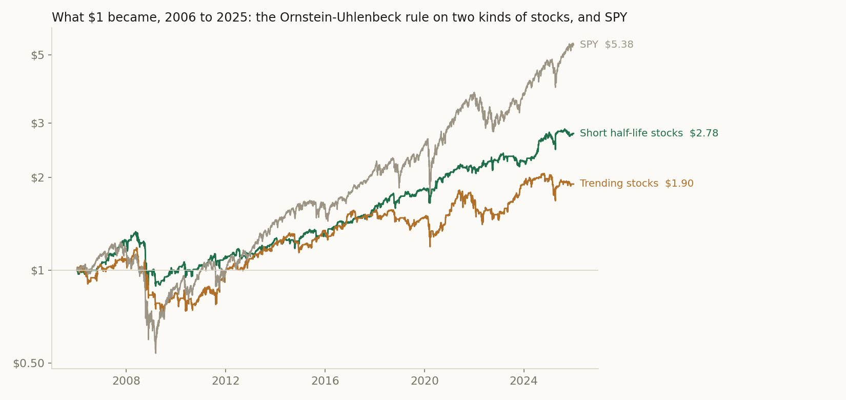
Did the rule do better on the short half-life stocks? Yes. With the same rule and the same money, $1 became $2.78 on the short half-life stocks and $1.90 on the trending stocks (Figure 3). In the 2008 crash the short half-life portfolio fell 33% at its worst, the trending portfolio 41%.
Why? In both groups a winning trade made about two thirds of what a losing trade lost. The trending stocks swung about a third more, so on them both the wins and the losses were larger, by the same proportion. The difference was how often the trades won: 67 in 100 on the short half-life stocks and 64 in 100 on the trending stocks. Measured against the size of a losing trade, an average trade on the short half-life stocks earned about twice as much as one on the trending stocks.
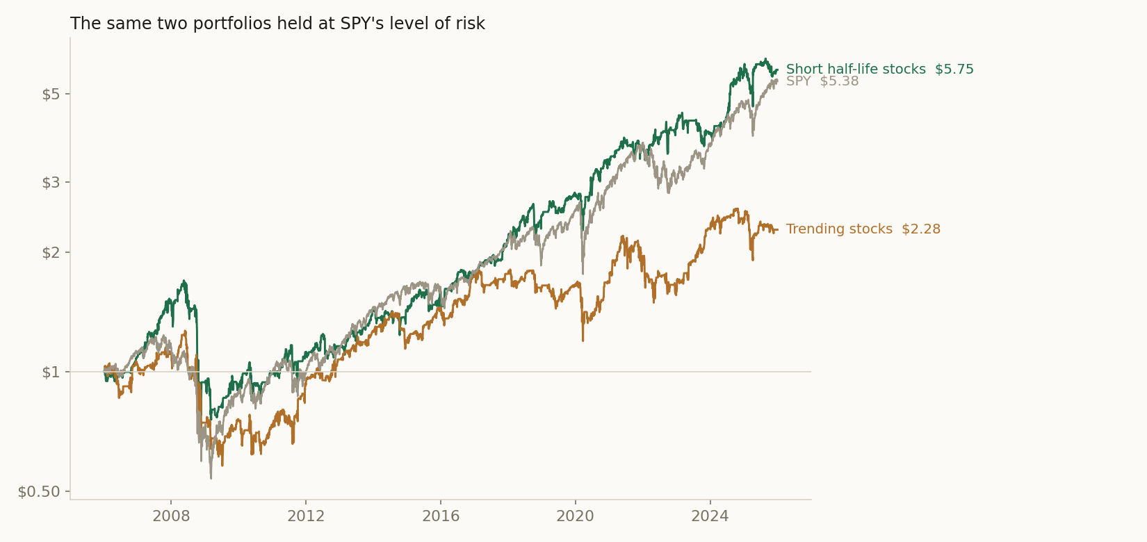
How does it compare with SPY? The rule buys a stock only when its price is far below its mean and sells it once the price is back near the mean, so about three quarters of the money waited in cash. As it ran, it made less than SPY, $2.78 against $5.38, and its worst fall, in the 2008 crash, was much smaller: 33% from its high, against 56% for SPY. Held at the same level of risk as SPY, with each stock's share nearly twice as big, the short half-life portfolio turned $1 into $5.75, against $5.38 for SPY, before trading costs (Figure 4).
Did the Kelly formula help? The Kelly formula is a well-known rule for deciding how much to bet; the mathematician Ed Thorp used it at the blackjack table. It puts more money on the stocks whose past trades won more often and whose wins were large next to their losses. It changed little here: half Kelly ended about where equal shares did, and full Kelly moved up and down more. Most stocks made about nine trades a year, too few for the formula, so most of the time it gave them an equal share.
1 Methodology, in detail (click to open)
1 Methodology
The stocks. The S&P 500 as its members stood on each first trading day of January and July, 2006 to 2025. Every member with a reliable price history in our data is measured.
The half-life. For each stock: the logarithm of the past year of daily closes, minus its least-squares straight line; an AR(1) fit to what is left; and the half-life −ln(2) / ln(b) in trading days, where b is the AR(1) coefficient with Kendall's small-sample correction. When b is 1 or more there is no pull back to the line, and the half-life is set to its ceiling of 999 days. The trending portfolio ranks every stock half on a long half-life and half on the slope of the past year's line, and keeps the top five. The short half-life portfolio keeps the five shortest. For the six months after, the same measure is computed on the closes of the six months each stock was traded.
The rule. The Ornstein-Uhlenbeck z-score with the 60 trading days and the −1.25 and −0.5 lines of Avellaneda and Lee (2010), who applied them to each stock's moves net of its sector fund, long and short, and only to stocks that reverted fast. Here the rule trades each stock's own price, long only. Every day it fits the model to the past 60 trading days, estimating the mean and the stationary standard deviation, the spread the model settles into, and measures the close's distance from the mean in those standard deviations. It buys when the z-score falls below −1.25, sells when it rises above −0.5, and stops out below −3.5, the platform card's own stop, after which it does not buy again until the z-score is back above −3.5. The trade is filled at that close. The same settings for every stock in every test. The platform's record of each test lists an optimizer card for both portfolios and describes the settings as optimized on a grid; that grid held a single setting, 60 days and −1.25, so it chose nothing. It is in the circuit only to hand the Kelly sizing each stock's trades over the year before.
Sizing. Equal shares: each of the five holds a fifth of the money while in a trade. Kelly: each stock's share is its win rate minus its loss rate divided by its win/loss size ratio, from its trades at the same settings over the year before; half Kelly takes half of that. A stock with fewer than 12 trades or fewer than 2 losses in that year gets a fifth. The Kelly portfolios could hold up to twice their money in stocks. Each sizing ran as its own set of the same 40 tests, each written down and locked before it ran. The record on this page is the equal-share set; the two Kelly sets are kept as separate studies.
The tests. Each six-month test starts in cash. No trading costs, no interest on cash, prices without dividends. The figures join the 40 tests end to end from $1 at the first close of 2006 to the last close of 2025. Where a test ends before the next one's first close, the day between is carried with what each portfolio held at the previous close, and SPY with its own closes, as in our recent papers. The page's record further down computes its own figures on the 40 tests as recorded, which leave out the day between tests, so its figures for SPY and the trending stocks are slightly lower than in this paper.
SPY's level of risk. Each portfolio's daily return is multiplied by one number: SPY's standard deviation of daily returns over the portfolio's own, over the twenty years. On days when the scaled shares add up to more than all of the money, the part above it is borrowed.
Costs. For each trade, the stock's share of the money times 0.1%, once for the purchase and once for the sale, summed and divided by twenty years; at SPY's level of risk, times the multiplier. The tests themselves charge no costs, which is what the page's record means by costs not being modelled; the after-cost figures in this paper are worked out afterwards from the trades.
Transaction costs are not modelled in this study; all results are gross of costs.
2 Results
Findings
The two groups of stocks. In every one of the 40 tests, the middle stock of the short half-life five had a half-life of four to nine trading days in the year before. The ones picked most often included power and gas companies (NiSource, Dominion Energy, FirstEnergy), TJX (the owner of TJ Maxx), ExxonMobil and Mastercard. The trending stocks were often fast-growing companies: AMD and NVIDIA were among them in six tests each, Apple and Meta in four. In more than half of the tests, the middle trending stock showed no pull back at all within the year.
The six months after. Measured again on the six months each stock was traded, the middle short half-life stock had a half-life of about 12 trading days and the middle trending stock about 15. Made-up random prices with no pull at all give about 16 days on six months. On one year, the five shortest out of several hundred such random prices come out at 5 to 8 trading days, about what the short half-life stocks showed when they were picked.
Growth. Over the twenty years the short half-life portfolio grew 5.2% a year, the trending portfolio 3.3% and SPY 8.8% (Figure 3 and the yearly tables below). The short half-life portfolio did better than the trending portfolio in 23 of the 40 six-month tests.
The trades. The short half-life portfolio made 913 trades and the trending portfolio 844. On the short half-life stocks 67 in 100 made money, on the trending stocks 64 in 100. A winning trade made 3.2% on average on the short half-life stocks and 4.2% on the trending stocks; a losing trade lost 4.7% and 6.3%. The worst single trade lost 43% and 56%.
The stocks themselves. In the six months they were traded, the middle short half-life stock swung 25% a year and the middle trending stock 34%. Over those six months the middle short half-life stock rose 2.4% and the middle trending stock 5.9%; the rule, which waits for prices to fall below their mean, held little of that rise.
Time in cash. Each stock was held on about a quarter of the days. On an average day about three quarters of the money was in cash, which earns nothing in these tests.
When the market fell and when it rose. In the six-month tests in which SPY fell, the short half-life portfolio did better than SPY 9 times out of 10. In the tests in which SPY rose, it did better 7 times out of 30.
At SPY's level of risk (Figure 4). With each stock's share made 1.88 times bigger, the short half-life portfolio moved up and down as much as SPY. It grew 9.1% a year, against 8.8% for SPY, and fell 55% at its worst, against 56%. On most days the bigger shares fitted into the money the portfolio had. On 16% of the days, when three or more stocks were in a trade at once, it would have borrowed, on an average day 5% of its money.
The Kelly formula. With half Kelly, $1 became $2.90 on the short half-life stocks, and with full Kelly $3.01, against $2.78 with equal shares. At SPY's level of risk, full Kelly grew 7.9% a year, less than equal shares. On the trending stocks both did slightly worse than equal shares. Only about one stock in twenty had enough past trades for the formula to set its share; the others got an equal share.
Trading costs. At 0.1% of every purchase and every sale, costs would take about 1.8 percentage points a year from the short half-life portfolio as it ran, and about 3.4 at SPY's level of risk. The table of the three sizings shows every line after these costs.
2.1 Headline
Table 1. Each year's return before trading costs, prices without dividends. Each year runs from the last close of the year before; 2006 starts at its first close. At SPY's risk: each stock's share 1.88 times bigger, so the portfolio moves up and down as much as SPY.
| Year | Short half-life | Trending | SPY | Short half-life at SPY's risk |
|---|---|---|---|---|
| 2006 | +4.9% | +3.3% | +11.8% | +9.2% |
| 2007 | +18.8% | +4.6% | +3.2% | +37.6% |
| 2008 | −20.2% | −23.1% | −38.3% | −37.4% |
| 2009 | −1.2% | +1.5% | +23.5% | −3.3% |
| 2010 | +5.4% | −2.0% | +12.8% | +8.8% |
| 2011 | +7.1% | +19.2% | −0.2% | +12.9% |
| 2012 | +2.3% | +10.7% | +13.5% | +3.8% |
| 2013 | +11.6% | +11.7% | +29.7% | +22.6% |
| 2014 | +0.6% | −3.2% | +11.3% | +0.7% |
| 2015 | +5.8% | +13.3% | −0.8% | +10.7% |
Table 2. Each year's return before trading costs, prices without dividends. Each year runs from the last close of the year before; 2006 starts at its first close. At SPY's risk: each stock's share 1.88 times bigger, so the portfolio moves up and down as much as SPY.
| Year | Short half-life | Trending | SPY | Short half-life at SPY's risk |
|---|---|---|---|---|
| 2016 | +5.8% | +13.9% | +9.6% | +10.6% |
| 2017 | +10.9% | +1.4% | +19.4% | +21.2% |
| 2018 | +8.7% | −5.1% | −6.3% | +15.9% |
| 2019 | +7.2% | +1.3% | +28.8% | +13.8% |
| 2020 | +11.3% | +2.1% | +16.2% | +20.5% |
| 2021 | +5.6% | +10.6% | +27.0% | +10.4% |
| 2022 | +7.0% | −12.3% | −19.5% | +12.6% |
| 2023 | −2.3% | +29.0% | +24.3% | −4.7% |
| 2024 | +19.4% | +2.6% | +23.3% | +38.8% |
| 2025 | +2.8% | −2.3% | +16.4% | +3.6% |
| A year, 2006 to 2025 | 5.2% | 3.3% | 8.8% | 9.1% |
| $1 became | $2.78 | $1.90 | $5.38 | $5.75 |
Table 3. Before trading costs unless marked. Costs at 0.1% of every purchase and every sale, worked out from the trades. Prices without dividends; no interest on cash.
| $1 became | A year | Worst fall | At SPY's risk, a year | Same, after costs | |
|---|---|---|---|---|---|
| Short half-life, equal shares | $2.78 | 5.2% | 33% | 9.1% | 5.7% |
| Short half-life, half Kelly | $2.90 | 5.5% | 32% | 9.1% | 5.8% |
| Short half-life, full Kelly | $3.01 | 5.7% | 38% | 7.9% | 4.9% |
| Trending, equal shares | $1.90 | 3.3% | 41% | 4.2% | 1.7% |
| Trending, half Kelly | $1.81 | 3.0% | 42% | 3.8% | 1.4% |
| Trending, full Kelly | $1.81 | 3.0% | 45% | 3.7% | 1.3% |
| SPY | $5.38 | 8.8% | 56% | 8.8% | 8.8% |
Table 4. How many of the 40 six-month tests had each stock among the five (3 or more; several more stocks share the last count).
| Short half-life | Six-month tests | Trending | Six-month tests |
|---|---|---|---|
| NiSource (NI) | 4 | AMD | 6 |
| TJX | 3 | NVIDIA (NVDA) | 6 |
| ExxonMobil (XOM) | 3 | Apple (AAPL) | 4 |
| Cencora (COR) | 3 | Meta (META) | 4 |
| Mastercard (MA) | 3 | Hasbro (HAS) | 3 |
| Dominion Energy (D) | 3 | Archer-Daniels-Midland (ADM) | 3 |
| Aptiv (APTV) | 3 | Southwest Airlines (LUV) | 3 |
| FirstEnergy (FE) | 3 | Booking Holdings (BKNG) | 3 |
Sections 2.2 to 3, the full record: every year, every test, and how each one was run (click to open)
The registration names the two groups compared The five fastest to come back, traded by OU and The five slowest, tilted to rising, traded by OU; this paper calls them Short half-life stocks and Trending stocks.
2.2 Per-step results
| # | Out-of-sample window | Short half-life stocks SR | Trending stocks SR |
|---|---|---|---|
| 1 | 2006-01-03 → 2006-06-30 | -0.29 | -1.16 |
| 2 | 2006-07-03 → 2006-12-29 | 2.99 | 2.05 |
| 3 | 2007-01-03 → 2007-06-29 | 2.27 | -0.13 |
| 4 | 2007-07-02 → 2007-12-31 | 2.10 | 0.98 |
| 5 | 2008-01-02 → 2008-07-01 | 0.14 | -1.03 |
| 6 | 2008-07-01 → 2008-12-31 | -1.53 | -1.27 |
| 7 | 2009-01-02 → 2009-07-01 | -0.92 | -1.14 |
| 8 | 2009-07-01 → 2009-12-31 | 1.26 | 2.07 |
| 9 | 2010-01-04 → 2010-07-01 | 0.14 | -0.44 |
| 10 | 2010-07-01 → 2010-12-31 | 0.85 | 0.79 |
| 11 | 2011-01-03 → 2011-07-01 | 1.81 | 0.66 |
| 12 | 2011-07-01 → 2011-12-30 | 0.01 | 1.26 |
| 13 | 2012-01-03 → 2012-06-29 | 1.89 | 0.05 |
| 14 | 2012-07-02 → 2012-12-31 | -0.70 | 1.67 |
| 15 | 2013-01-02 → 2013-07-01 | 0.84 | 1.87 |
| 16 | 2013-07-01 → 2013-12-31 | 3.42 | 1.20 |
| 17 | 2014-01-02 → 2014-07-01 | -0.36 | 1.21 |
| 18 | 2014-07-01 → 2014-12-31 | 0.44 | -2.00 |
| 19 | 2015-01-02 → 2015-07-01 | 1.99 | 1.22 |
| 20 | 2015-07-01 → 2015-12-31 | 0.11 | 1.98 |
| 21 | 2016-01-04 → 2016-07-01 | 1.65 | 0.76 |
| 22 | 2016-07-01 → 2016-12-30 | -0.03 | 2.25 |
| 23 | 2017-01-03 → 2017-06-30 | 1.50 | -0.40 |
| 24 | 2017-07-03 → 2017-12-29 | 2.15 | 1.00 |
| 25 | 2018-01-02 → 2018-06-29 | 1.30 | -0.32 |
| 26 | 2018-07-02 → 2018-12-31 | 0.53 | -0.68 |
| 27 | 2019-01-02 → 2019-07-01 | 0.78 | -1.28 |
| 28 | 2019-07-01 → 2019-12-31 | 2.21 | 1.58 |
| 29 | 2020-01-02 → 2020-07-01 | 0.61 | -0.88 |
| 30 | 2020-07-01 → 2020-12-31 | 1.58 | 2.47 |
| 31 | 2021-01-04 → 2021-07-01 | 2.51 | 2.77 |
| 32 | 2021-07-01 → 2021-12-31 | -0.18 | -0.39 |
| 33 | 2022-01-03 → 2022-07-01 | 0.46 | -0.69 |
| 34 | 2022-07-01 → 2022-12-30 | 0.96 | -1.12 |
| 35 | 2023-01-03 → 2023-06-30 | 0.30 | 2.26 |
| 36 | 2023-07-03 → 2023-12-29 | -0.78 | 2.85 |
| 37 | 2024-01-02 → 2024-07-01 | 1.98 | 0.79 |
| 38 | 2024-07-01 → 2024-12-31 | 2.22 | -0.43 |
| 39 | 2025-01-02 → 2025-07-01 | 0.52 | 0.03 |
| 40 | 2025-07-01 → 2025-12-31 | -0.69 | -0.54 |
2.3 Search accounting
No search record exists for this design. It was not promoted from a recorded evolving search, so the number of alternatives tried before it, on paper, in another tool, or in the author's head, is unknown. Unknown is a different fact from one: a study with no lineage is not a strategy with one trial, it is a strategy with an unrecorded number of them. Accordingly no count of alternatives tried is claimed, and nothing in this paper is corrected for a search that was never recorded; the number that stands is the raw out-of-sample result plus this disclosure. The registered per-step record below (§4) still guarantees each window's hypothesis was hashed and registered before that window was scored.
2.4 The comparison
Both arms trade the same registered windows, so their returns can be PAIRED: inside each window the two return series are inner-joined date by date and the difference rShort half-life stocks − rTrending stocks is the object under test. Because this is ONE pre-declared contrast, frozen at registration before any window was scored, the paired statistic needs no multiple-testing deflation, and the per-arm pooled numbers above are likewise uncorrected, because this design has no recorded search to correct against (§2.3). The paired contrast carries that gap differently from the arm levels: it was declared before each window ran and it is scored on the difference, so no window could be read first and scored after. What the timestamps cannot speak to is how this contrast came to be the declared one, which is the limit §2.3 states.
In the table: Arm A = Short half-life stocks · Arm B = Trending stocks.
| # | Window | Paired bars | Arm A | Arm B | Δ | Leader |
|---|---|---|---|---|---|---|
| 1 | 2006-01-04 → 2006-06-30 | 124 | -1.0% | -7.4% | +6.4 pp | Arm A |
| 2 | 2006-07-05 → 2006-12-29 | 125 | +5.9% | +11.6% | -5.7 pp | Arm B |
| 3 | 2007-01-04 → 2007-06-29 | 123 | +7.9% | -0.6% | +8.5 pp | Arm A |
| 4 | 2007-07-03 → 2007-12-31 | 126 | +10.1% | +4.6% | +5.5 pp | Arm A |
| 5 | 2008-01-03 → 2008-07-01 | 125 | +0.4% | -6.6% | +7.1 pp | Arm A |
| 6 | 2008-07-02 → 2008-12-31 | 127 | -20.0% | -18.3% | -1.7 pp | Arm B |
| 7 | 2009-01-05 → 2009-07-01 | 124 | -6.4% | -9.6% | +3.2 pp | Arm A |
| 8 | 2009-07-02 → 2009-12-31 | 127 | +5.6% | +12.3% | -6.7 pp | Arm B |
| 9 | 2010-01-05 → 2010-07-01 | 124 | +0.5% | -5.6% | +6.1 pp | Arm A |
| 10 | 2010-07-02 → 2010-12-31 | 127 | +3.5% | +4.2% | -0.7 pp | Arm B |
| 11 | 2011-01-04 → 2011-07-01 | 125 | +6.8% | +3.8% | +3.1 pp | Arm A |
| 12 | 2011-07-05 → 2011-12-30 | 126 | -0.3% | +14.0% | -14.3 pp | Arm B |
| 13 | 2012-01-04 → 2012-06-29 | 124 | +5.5% | +0.0% | +5.5 pp | Arm A |
| 14 | 2012-07-03 → 2012-12-31 | 124 | -3.3% | +8.7% | -12.1 pp | Arm B |
| 15 | 2013-01-03 → 2013-07-01 | 124 | +3.2% | +6.7% | -3.5 pp | Arm B |
| 16 | 2013-07-02 → 2013-12-31 | 127 | +8.2% | +4.7% | +3.5 pp | Arm A |
| 17 | 2014-01-03 → 2014-07-01 | 124 | -1.1% | +5.8% | -6.9 pp | Arm B |
| 18 | 2014-07-02 → 2014-12-31 | 127 | +1.7% | -8.8% | +10.4 pp | Arm A |
| 19 | 2015-01-05 → 2015-07-01 | 124 | +5.5% | +6.1% | -0.6 pp | Arm B |
| 20 | 2015-07-02 → 2015-12-31 | 127 | +0.3% | +6.7% | -6.4 pp | Arm B |
| 21 | 2016-01-05 → 2016-07-01 | 125 | +7.0% | +4.0% | +3.0 pp | Arm A |
| 22 | 2016-07-05 → 2016-12-30 | 126 | -0.2% | +9.8% | -10.1 pp | Arm B |
| 23 | 2017-01-04 → 2017-06-30 | 124 | +3.0% | -2.6% | +5.7 pp | Arm A |
| 24 | 2017-07-05 → 2017-12-29 | 125 | +7.0% | +3.7% | +3.3 pp | Arm A |
| 25 | 2018-01-03 → 2018-06-29 | 124 | +4.9% | -1.8% | +6.7 pp | Arm A |
| 26 | 2018-07-03 → 2018-12-31 | 125 | +3.0% | -3.7% | +6.7 pp | Arm A |
| 27 | 2019-01-03 → 2019-07-01 | 124 | +2.0% | -5.1% | +7.0 pp | Arm A |
| 28 | 2019-07-02 → 2019-12-31 | 127 | +5.1% | +6.7% | -1.7 pp | Arm B |
| 29 | 2020-01-03 → 2020-07-01 | 125 | +4.3% | -10.6% | +14.9 pp | Arm A |
| 30 | 2020-07-02 → 2020-12-31 | 127 | +7.5% | +13.9% | -6.4 pp | Arm B |
| 31 | 2021-01-05 → 2021-07-01 | 124 | +7.5% | +17.7% | -10.2 pp | Arm B |
| 32 | 2021-07-02 → 2021-12-31 | 127 | -0.8% | -5.4% | +4.6 pp | Arm A |
| 33 | 2022-01-04 → 2022-07-01 | 124 | +2.1% | -7.3% | +9.4 pp | Arm A |
| 34 | 2022-07-05 → 2022-12-30 | 126 | +5.1% | -6.0% | +11.1 pp | Arm A |
| 35 | 2023-01-04 → 2023-06-30 | 123 | +0.9% | +13.1% | -12.1 pp | Arm B |
| 36 | 2023-07-05 → 2023-12-29 | 125 | -3.4% | +13.6% | -17.0 pp | Arm B |
| 37 | 2024-01-03 → 2024-07-01 | 124 | +6.0% | +4.5% | +1.5 pp | Arm A |
| 38 | 2024-07-02 → 2024-12-31 | 127 | +13.3% | -1.9% | +15.2 pp | Arm A |
| 39 | 2025-01-03 → 2025-07-01 | 122 | +4.3% | -0.7% | +5.0 pp | Arm A |
| 40 | 2025-07-02 → 2025-12-31 | 127 | -2.3% | -1.7% | -0.6 pp | Arm B |
Paired Sharpe of the difference track: 0.14 · block bootstrap (2000 paths, block 10, seed 1234): P(Short half-life stocks beats Trending stocks) = 74.9%.
Window win-rate. Short half-life stocks led 23 of 40 windows (57.5%), Trending stocks led 17, and the mean window gap of +0.91 pp points the same way. Widest single window: 2023 at -17.0 pp.
| Period | Windows | Short half-life stocks | Trending stocks | Mean gap | Short half-life stocks led |
|---|---|---|---|---|---|
| All windows | 40 | +2.73% | +1.81% | +0.91 pp | 23/40 |
| Before 2010 | 8 | +0.31% | -1.77% | +2.08 pp | 5/8 |
| 2010 onward | 32 | +3.33% | +2.71% | +0.62 pp | 18/32 |
3 The circuit
The strategy is a circuit of platform primitives, frozen when the study is registered. Below is the circuit as wired on the canvas, the objective it encodes and how the search runs through it, followed by the mathematics each primitive actually computes, the same formulas the execution engine runs. The complete parameterisation is preserved in the study ledger (Appendix A).
The sentence below is the registration record, generated when the circuit was registered and printed verbatim; the authored description of the design is Section 1.
A COMPARATIVE study: The five fastest to come back, traded by OU vs The five slowest, tilted to rising, traded by OU, walked on the same registered out-of-sample windows. The five fastest to come back, traded by OU: S&P 500, the highest 5 by composite score (low OU half-life), traded via OU Z-Score signal, with its settings optimized in-sample over the year before the anchor (the best Sharpe ratio on a grid, each name its own), and forward-tested out-of-sample from the anchor: the settings are frozen at the anchor. The five slowest, tilted to rising, traded by OU: S&P 500, the highest 5 by composite score (high OU half-life, high trend slope), traded via OU Z-Score signal, with its settings optimized in-sample over the year before the anchor (the best Sharpe ratio on a grid, each name its own), and forward-tested out-of-sample from the anchor: the settings are frozen at the anchor. The arms differ in: 2 nodes across 3 recorded settings: Composite Σ, Directions (criterion:low|high, …): ou_half_life:low → ou_half_life:high, trend_slope:high; Composite Σ, Weights (criterion:weight, …): ou_half_life:100 → ou_half_life:50, trend_slope:50; Trend Slope, added in The five slowest, tilted to rising, traded by OU. NOTE: with more than one difference, an out-of-sample gap cannot be attributed to any single change. The contrast under test: whether The five fastest to come back, traded by OU generates better risk-adjusted returns than The five slowest, tilted to rising, traded by OU over the identical out-of-sample windows.
Every block in this study is a card from the platform's catalog: the S&P 500 as it stood on each day, the OU Half-Life card (and Trend Slope for the trending stocks) into the Composite and Top-N for the five, the OU Z-Score card with Avellaneda and Lee's buy and sell lines and the card's own stop, the Stochastic Optimizer set to those same settings only, so it searches nothing and only hands the Kelly sizing each stock's past trades, and the Stoch Forward Test for six months. You can rebuild every test and change any setting.
Envelopes show counts, ratios, dates, and the parameters the author chose. Full price and per-name data series are not republished: the underlying market data is licensed to QuanterLab. Point figures quoted in the prose, a named holding's return over a stated span, are summary facts derived from public market prices, not redistributed series.
The objective and the search
The five fastest to come back, traded by OU
| Universe | S&P 500 index constituents. |
|---|---|
| Selection | composite-scored across OU half-life → highest 5 kept by composite score. |
| Signal generation | OU Z-Score signal. |
| In-sample search | In-sample optimization via the Stochastic Optimizer: each name's best Sharpe ratio on a grid over the year before the anchor; sweeping lookback ∈ [60, 60] / 2 steps × z_entry ∈ [1.25, 1.25] / 2 steps, traded unchanged from the anchor. |
| Validation & out-of-sample | stochastic forward test (6m horizon from the anchor). |
The five slowest, tilted to rising, traded by OU
| Selection | composite-scored across OU half-life, Trend slope (252 days) → highest 5 kept by composite score. |
|---|
Every other specification row is identical to The five fastest to come back, traded by OU's table above.
What differs between the arms, 2 differences; more than one thing changes at once:
- paramComposite Σ, Directions (criterion:low|high, …): ou_half_life:low → ou_half_life:high, trend_slope:high
- paramComposite Σ, Weights (criterion:weight, …): ou_half_life:100 → ou_half_life:50, trend_slope:50
- addedTrend Slope, added in The five slowest, tilted to rising, traded by OU
Reader's note. With 3 settings changed at once across 2 nodes, an out-of-sample gap between the arms cannot be attributed to any single change, the arms are compared as whole packages, and any causal reading of one ingredient is unsupported by this design.
No transaction-cost elements are wired into this circuit; results are gross of costs.
Show the mathematics, 9 primitives, formulas and parity notes
3.1 Universe
The starting set of tickers, resolved point-in-time from the index change-log, so names delisted or removed later still compete on the dates they traded.
Before any math, you need a list of stocks. An index preset (S&P 500, Nasdaq-100, Dow 30) is reconstructed as it stood ON your anchor date by replaying the historical add/drop change-log backwards, so a 2018 backtest sees the 2018 membership, not today's winners.
Start from today's constituents and un-apply every membership change after the anchor t:
\mathcal{U}(t) = \mathcal{U}_{\text{now}} \;\ominus\; \{\text{adds after } t\} \;\oplus\; \{\text{drops after } t\}3.2 Price Loader
Bulk OHLCV fetch for the whole universe, point-in-time, no future bars.
Momentum, volatility, trend, every price-based metric needs history. This loads open/high/low/close/volume for all names in parallel, clipped so nothing after the anchor can leak in. The lookback window is derived automatically from the deepest metric you wired.
It loads exactly enough history for the hungriest downstream metric plus a warm-up buffer:
W = \max_k(\text{lookback}_k) + \text{buffer}, \qquad \text{bars} \le \text{anchor } t3.3 Filter Ou Halflife
Ornstein–Uhlenbeck half-life, how many days a deviation takes to decay by half.
First remove the long-term drift (an OLS trend line fitted to log-price), then fit an AR(1) to what remains. The autoregressive coefficient β says how fast deviations from trend get pulled back; convert it to a half-life in days. Roughly 5–40 days is the tradeable sweet spot for mean reversion.
\log P_t = a + b\,t + \varepsilon_t \quad\Longrightarrow\quad x_t = \log P_t - (a + b\,t)x_t = \alpha + \beta\,x_{t-1} + \varepsilon_t\text{half-life} = \frac{\ln 2}{\lvert \ln \beta \rvert}3.4 Composite Score
The composite, turn many metrics into one 0–100 score per stock.
Each wired metric is ranked across all stocks into a 0–100 percentile (you choose whether high or low is "good"), then the percentiles are weight-averaged. Ranking instead of raw values means no single unit dominates and outliers can't blow it up. It scores; it does not drop.
\text{pct}_k(i) = 100 \cdot \frac{\operatorname{rank}_k(i)}{N}\text{score}_i = \frac{\sum_k w_k\,\text{pct}_k(i)}{\sum_k w_k} \in [0,100]3.5 Top N
Keep the best N, rank, then cut.
Sort the survivors by the Composite Σ (or, if none is wired, the last metric in the chain) and keep the top (or bottom) N. The final narrowing from a scored list to a committed basket.
\text{Top-}N = \{\, i : \operatorname{rank}(\text{score}_i) \le N \,\}N = \operatorname{round}(f \cdot n_{\text{ranked}})\text{kept} = \{\, i \in H : \operatorname{rank}_i \le K \,\} \;\cup\; \text{best ranked } i \notin H \text{ up to } N3.6 Stoch Ou Zscore
Ornstein–Uhlenbeck z-score, how stretched is the spring right now?
Detrend log-price and model the residual as a spring pulled back toward its mean. The z-score says how many standard deviations the spring is stretched; you fade the extremes and exit near the mean.
dx_t = \theta(\mu - x_t)\,dt + \sigma\,dW_t \quad\Longleftrightarrow\quad x_t = \alpha + \beta\,x_{t-1} + \varepsilon_tz_t = \frac{x_t - \mu}{\sigma}\ \ (\text{clipped }\pm 5), \qquad \text{half-life} = \frac{\ln 2}{\lvert\ln\beta\rvert}3.7 Stochastic Optimize
Optimize an OU / Kalman rule on the past, once, and hand it on.
The grid search of the stochastic lane as a card of its own: for each name it tries every pair of the two chosen settings (for OU, the look back and the entry threshold) on that name's own prices over the window that ends at the anchor, and keeps the pair with the best Sharpe ratio. The Stoch Forward Test then trades those settings, unchanged, from the anchor on: one optimization on the past, no folds, and everything after the anchor is out of sample.
\boldsymbol\theta^*_i = \arg\max_{\boldsymbol\theta\in\text{grid}}\,\text{Sharpe}_{[\,t_0 - W,\;t_0\,]}\big(\text{name}_i;\boldsymbol\theta\big)3.8 Stochastic Forward
Forward-test an OU / Kalman rule on unseen data.
Takes the validated stochastic configuration and trades it bar-by-bar on a forward window it has never seen, producing the out-of-sample equity curve, trades and statistics.
\text{enter at } \lvert z_t\rvert > z_{\text{entry}},\ \ \text{exit at } \lvert z_t\rvert < z_{\text{exit}}3.9 Filter Trend Slope
Trend slope, the annualized direction and steepness.
The slope of a straight line fitted to log-price, scaled to a yearly rate. Signed: strongly positive is a powerful uptrend, negative a downtrend. The line is fitted over about six months unless you set the window. With "Steadiness counts" on, it is the ranking of Andreas Clenow's Stocks on the Move: the yearly speed times how straight the line is, so a steady climb ranks above a jumpy one of the same speed.
\text{slope}_{\text{ann}} = b \times 252, \qquad \log P_\tau = a + b\,\tau\text{score} = \left(e^{\,252\,b} - 1\right) \times R^24 Discussion
4.1 Interpretation
The Ornstein-Uhlenbeck rule is only as good as the stocks it is given. Pointed at the stocks with the shortest half-life, it did better than pointed at trending stocks, with every way of sizing the trades, and its trades won more often. In the six months they were traded, though, the two groups' half-lives were close to what random prices give, so this test cannot say how much of the difference comes from the half-life itself and how much from staying away from trending stocks.
As it ran, the rule made less than SPY, because it waits in cash until a price is far below its mean. That waiting also kept it out of about half of the 2008 fall. Held at SPY's level of risk, the short half-life portfolio ended ahead of SPY, before trading costs.
The model behind the rule is old and plain: a level, a pull and a spread, estimated from recent prices. We used the buy and sell lines of the best-known practitioners' study of it, the same for every stock, and did not search for the settings that would have done best in the past. The results here are what those standard settings did.
The Kelly formula added little, because a stock traded this way makes too few trades in a year for the formula to size it.
For a reader, the practical point is that the same rule did much better on the stocks with the shortest half-life than on trending stocks, and that a half-life measured on one year should be read with care, since on one year of prices a short half-life can come from chance alone.
4.2 Limitations
Forty tests of six months each are not many. A few very good and very bad years decide the comparison at SPY's level of risk; the yearly tables show them.
The half-life is measured on one year of prices. On random prices with no pull at all, the five shortest out of several hundred come out at 5 to 8 trading days, about what the short half-life stocks showed, so a short half-life on one year can come from chance alone. In the six months they were traded, their half-lives were longer than when they were picked.
We did not run the rule on five stocks picked at random, or simply hold the same five stocks. So we cannot separate the effect of the half-life from the effect of avoiding trending stocks or of picking calmer companies.
No trading costs are charged inside the tests. We worked them out afterwards from the number of trades. At 0.1% of every purchase and sale, the short half-life portfolio at SPY's level of risk grows about 5.7% a year instead of 9.1%.
Each purchase and sale happens at the closing price of the day the rule decides. A trader who can only trade the next day would get different prices.
Dividends and interest on cash are left out, and they pull in opposite directions. Dividends would favour SPY, which paid about 2% a year. Interest on cash would favour the short half-life portfolio, which held a lot of cash.
The bigger share used to match SPY's level of risk is one number for the whole twenty years, found afterwards. On the days it needed to borrow, we assumed borrowing at 2% a year, which costs about 0.1 of a percentage point a year.
Our price data has no prices for many companies that later left the S&P 500: about a third of the index in 2006, under a tenth from 2015. Such a company can never be picked, so both portfolios probably look better here than they would with every company included.
We tried one setting of each part of the rule and five stocks per portfolio. Other choices would give other results.
Try it yourself
Every test in this paper can be run again on quanterlab.com, and you can change any setting. Open it in the lab and try, for example:
• five stocks picked at random, to see how much the half-life adds;
• ten or twenty stocks instead of five;
• a buy line further from the mean, which trades less often;
• trading on the next day's price instead of the same day's.
Or ask the lab assistant to build a version for you, in your own words, and watch it build the test step by step. On Practitioner and Research, a version you like can start live on paper, with a note on it every morning.
References
- Uhlenbeck, G. E. and Ornstein, L. S. (1930). On the theory of the Brownian motion. Physical Review 36(5), 823-841. The process, first written down for the speed of particles in a liquid. https://doi.org/10.1103/PhysRev.36.823
- Avellaneda, M. and Lee, J.-H. (2010). Statistical arbitrage in the US equities market. Quantitative Finance 10(7), 761-782. The 60 trading days and the −1.25 and −0.5 lines, applied there to stocks' moves net of their sector funds, long and short, and only to stocks that reverted fast. https://doi.org/10.1080/14697680903124632
- Chan, E. P. (2013). Algorithmic Trading: Winning Strategies and Their Rationale. Wiley. The half-life of mean reversion as a way to choose what to trade.
- Kelly, J. L. (1956). A new interpretation of information rate. Bell System Technical Journal 35(4), 917-926. The betting formula. https://doi.org/10.1002/j.1538-7305.1956.tb03809.x
- Thorp, E. O. (2006). The Kelly criterion in blackjack, sports betting and the stock market. Handbook of Asset and Liability Management, volume 1, 385-428. How the formula went from the card table to the stock market.
- Moreira, A. and Muir, T. (2017). Volatility-managed portfolios. Journal of Finance 72(4), 1611-1644. Comparing portfolios at the same level of risk.
Appendix A Reproducibility in QuanterLab
Each step is backed by a frozen run report. The study is re-derivable from the ledger below.
| # | Commit | Report | Anchor | OOS window |
|---|---|---|---|---|
| 1 | aff4a024e084 | 15008 | 2006-01-01 | 2006-01-03 → 2006-06-30 |
| 2 | 2f72ced88691 | 15009 | 2006-07-01 | 2006-07-03 → 2006-12-29 |
| 3 | 0b5357a69c74 | 15010 | 2007-01-01 | 2007-01-03 → 2007-06-29 |
| 4 | b6da482633f9 | 15011 | 2007-07-01 | 2007-07-02 → 2007-12-31 |
| 5 | 9eed19043844 | 15012 | 2008-01-01 | 2008-01-02 → 2008-07-01 |
| 6 | a47ce10a49f1 | 15013 | 2008-07-01 | 2008-07-01 → 2008-12-31 |
| 7 | 93adf5aa6961 | 15014 | 2009-01-01 | 2009-01-02 → 2009-07-01 |
| 8 | 07183de7dd20 | 15015 | 2009-07-01 | 2009-07-01 → 2009-12-31 |
| 9 | c6739ee86627 | 15016 | 2010-01-01 | 2010-01-04 → 2010-07-01 |
| 10 | 995a87c01dd3 | 15017 | 2010-07-01 | 2010-07-01 → 2010-12-31 |
| 11 | d56cb019255c | 15018 | 2011-01-01 | 2011-01-03 → 2011-07-01 |
| 12 | 657d3a84a433 | 15019 | 2011-07-01 | 2011-07-01 → 2011-12-30 |
| 13 | 1c160ba4ccb8 | 15020 | 2012-01-01 | 2012-01-03 → 2012-06-29 |
| 14 | e7ef1f951405 | 15021 | 2012-07-01 | 2012-07-02 → 2012-12-31 |
| 15 | 00bbf3b9034d | 15022 | 2013-01-01 | 2013-01-02 → 2013-07-01 |
| 16 | 1a81cd76e44d | 15023 | 2013-07-01 | 2013-07-01 → 2013-12-31 |
| 17 | 3a5539b2a962 | 15024 | 2014-01-01 | 2014-01-02 → 2014-07-01 |
| 18 | b7a62b35f2eb | 15025 | 2014-07-01 | 2014-07-01 → 2014-12-31 |
| 19 | 182b3d0dcbc6 | 15026 | 2015-01-01 | 2015-01-02 → 2015-07-01 |
| 20 | fa68f6090af9 | 15027 | 2015-07-01 | 2015-07-01 → 2015-12-31 |
| 21 | 623316258066 | 15028 | 2016-01-01 | 2016-01-04 → 2016-07-01 |
| 22 | 75941afa1e97 | 15029 | 2016-07-01 | 2016-07-01 → 2016-12-30 |
| 23 | abc6aeb8b9a4 | 15030 | 2017-01-01 | 2017-01-03 → 2017-06-30 |
| 24 | 7ea970f35efb | 15031 | 2017-07-01 | 2017-07-03 → 2017-12-29 |
| 25 | f883896c01e9 | 15032 | 2018-01-01 | 2018-01-02 → 2018-06-29 |
| 26 | 97bd2df13632 | 15033 | 2018-07-01 | 2018-07-02 → 2018-12-31 |
| 27 | aade4e3989c3 | 15034 | 2019-01-01 | 2019-01-02 → 2019-07-01 |
| 28 | f59dc67d3344 | 15035 | 2019-07-01 | 2019-07-01 → 2019-12-31 |
| 29 | 20942be69373 | 15036 | 2020-01-01 | 2020-01-02 → 2020-07-01 |
| 30 | 6372adb3e320 | 15037 | 2020-07-01 | 2020-07-01 → 2020-12-31 |
| 31 | 5d5cf7abb6bf | 15038 | 2021-01-01 | 2021-01-04 → 2021-07-01 |
| 32 | 1e5082777acd | 15039 | 2021-07-01 | 2021-07-01 → 2021-12-31 |
| 33 | 0f2b5d878b4e | 15040 | 2022-01-01 | 2022-01-03 → 2022-07-01 |
| 34 | 1db3999886dd | 15041 | 2022-07-01 | 2022-07-01 → 2022-12-30 |
| 35 | c1c49d8b955e | 15042 | 2023-01-01 | 2023-01-03 → 2023-06-30 |
| 36 | 024ffa5acf41 | 15043 | 2023-07-01 | 2023-07-03 → 2023-12-29 |
| 37 | d874ce39dc4c | 15044 | 2024-01-01 | 2024-01-02 → 2024-07-01 |
| 38 | 6c47526fc65c | 15045 | 2024-07-01 | 2024-07-01 → 2024-12-31 |
| 39 | 764d5c917e75 | 15046 | 2025-01-01 | 2025-01-02 → 2025-07-01 |
| 40 | 4b0c4ab3b2c6 | 15047 | 2025-07-01 | 2025-07-01 → 2025-12-31 |
The methods the platform implements, for every study made on it, rest on these works.
- Gelman, A., & Loken, E. (2013). The garden of forking paths: Why multiple comparisons can be a problem, even when there is no “fishing expedition.” Working paper, Columbia University.
- Harvey, C. R., Liu, Y., & Zhu, H. (2016). … and the Cross-Section of Expected Returns. Review of Financial Studies, 29(1), 5–68. doi:10.1093/rfs/hhv059
- Lo, A. W. (2002). The Statistics of Sharpe Ratios. Financial Analysts Journal, 58(4), 36–52. doi:10.2469/faj.v58.n4.2453
Appendix A2 Registration record
What this record does and does not establish. Every window in this study is historical: the data existed before the study began, so this is sequential registration on past windows, not pre-registration in the clinical-trial sense, and no procedure could make it so. What the platform does enforce is order, each step's specification was frozen and hashed before that step was scored, and the walk cannot advance past a step that was never run or close one with a result registered for a different window. The two timestamp columns below are the evidence: read them together and each registration precedes its own run, and each run precedes the next registration. A study whose registrations all post-date its runs would show it here. Wall-clock spacing between registrations varies with the author's schedule and queue latency; the ordering, not the tempo, is the claim.
“A COMPARATIVE study: The five fastest to come back, traded by OU vs The five slowest, tilted to rising, traded by OU, walked on the same registered out-of-sample windows. The five fastest to come back, traded by OU: S&P 500, the highest 5 by composite score (low OU half-life), traded via OU Z-Score signal, with its settings optimized in-sample over the year before the anchor (the best Sharpe ratio on a grid, each name its own), and forward-tested out-of-sample from the anchor: the settings are frozen at the anchor. The five slowest, tilted to rising, traded by OU: S&P 500, the highest 5 by composite score (high OU half-life, high trend slope), traded via OU Z-Score signal, with its settings optimized in-sample over the year before the anchor (the best Sharpe ratio on a grid, each name its own), and forward-tested out-of-sample from the anchor: the settings are frozen at the anchor. The arms differ in: 2 nodes across 3 recorded settings: Composite Σ, Directions (criterion:low|high, …): ou_half_life:low → ou_half_life:high, trend_slope:high; Composite Σ, Weights (criterion:weight, …): ou_half_life:100 → ou_half_life:50, trend_slope:50; Trend Slope, added in The five slowest, tilted to rising, traded by OU. NOTE: with more than one difference, an out-of-sample gap cannot be attributed to any single change. The contrast under test: whether The five fastest to come back, traded by OU generates better risk-adjusted returns than The five slowest, tilted to rising, traded by OU over the identical out-of-sample windows.”
The same hypothesis was registered independently at every step, hashed before each step's out-of-sample window was scored:
| # | Anchor | Registered at (UTC) | Run completed (UTC) |
|---|---|---|---|
| 1 | 2006-01-01 | 2026-10-23 23:55:12 | 2026-10-23 23:56:16 |
| 2 | 2006-07-01 | 2026-10-23 23:56:16 | 2026-10-23 23:57:13 |
| 3 | 2007-01-01 | 2026-10-23 23:57:13 | 2026-10-23 23:58:02 |
| 4 | 2007-07-01 | 2026-10-23 23:58:02 | 2026-10-23 23:58:58 |
| 5 | 2008-01-01 | 2026-10-23 23:58:59 | 2026-10-23 23:59:55 |
| 6 | 2008-07-01 | 2026-10-23 23:59:55 | 2026-10-24 00:00:52 |
| 7 | 2009-01-01 | 2026-10-24 00:00:52 | 2026-10-24 00:01:56 |
| 8 | 2009-07-01 | 2026-10-24 00:01:56 | 2026-10-24 00:02:53 |
| 9 | 2010-01-01 | 2026-10-24 00:02:53 | 2026-10-24 00:03:58 |
| 10 | 2010-07-01 | 2026-10-24 00:03:58 | 2026-10-24 00:04:54 |
| 11 | 2011-01-01 | 2026-10-24 00:04:54 | 2026-10-24 00:05:51 |
| 12 | 2011-07-01 | 2026-10-24 00:05:51 | 2026-10-24 00:06:47 |
| 13 | 2012-01-01 | 2026-10-24 00:06:47 | 2026-10-24 00:07:44 |
| 14 | 2012-07-01 | 2026-10-24 00:07:44 | 2026-10-24 00:08:49 |
| 15 | 2013-01-01 | 2026-10-24 00:08:49 | 2026-10-24 00:09:45 |
| 16 | 2013-07-01 | 2026-10-24 00:09:45 | 2026-10-24 00:10:42 |
| 17 | 2014-01-01 | 2026-10-24 00:10:42 | 2026-10-24 00:11:38 |
| 18 | 2014-07-01 | 2026-10-24 00:11:38 | 2026-10-24 00:12:35 |
| 19 | 2015-01-01 | 2026-10-24 00:12:35 | 2026-10-24 00:13:39 |
| 20 | 2015-07-01 | 2026-10-24 00:13:39 | 2026-10-24 00:14:44 |
| 21 | 2016-01-01 | 2026-10-24 00:14:44 | 2026-10-24 00:15:49 |
| 22 | 2016-07-01 | 2026-10-24 00:15:49 | 2026-10-24 00:16:53 |
| 23 | 2017-01-01 | 2026-10-24 00:16:53 | 2026-10-24 00:17:58 |
| 24 | 2017-07-01 | 2026-10-24 00:17:58 | 2026-10-24 00:19:03 |
| 25 | 2018-01-01 | 2026-10-24 00:19:03 | 2026-10-24 00:20:10 |
| 26 | 2018-07-01 | 2026-10-24 00:20:10 | 2026-10-24 00:21:15 |
| 27 | 2019-01-01 | 2026-10-24 00:21:15 | 2026-10-24 00:22:20 |
| 28 | 2019-07-01 | 2026-10-24 00:22:20 | 2026-10-24 00:23:17 |
| 29 | 2020-01-01 | 2026-10-24 00:23:17 | 2026-10-24 00:24:21 |
| 30 | 2020-07-01 | 2026-10-24 00:24:21 | 2026-10-24 00:25:26 |
| 31 | 2021-01-01 | 2026-10-24 00:25:26 | 2026-10-24 00:26:33 |
| 32 | 2021-07-01 | 2026-10-24 00:26:33 | 2026-10-24 00:27:37 |
| 33 | 2022-01-01 | 2026-10-24 00:27:37 | 2026-10-24 00:28:42 |
| 34 | 2022-07-01 | 2026-10-24 00:28:42 | 2026-10-24 00:29:47 |
| 35 | 2023-01-01 | 2026-10-24 00:29:47 | 2026-10-24 00:30:52 |
| 36 | 2023-07-01 | 2026-10-24 00:30:52 | 2026-10-24 00:31:56 |
| 37 | 2024-01-01 | 2026-10-24 00:31:56 | 2026-10-24 00:33:01 |
| 38 | 2024-07-01 | 2026-10-24 00:33:01 | 2026-10-24 00:34:06 |
| 39 | 2025-01-01 | 2026-10-24 00:34:06 | 2026-10-24 00:35:10 |
| 40 | 2025-07-01 | 2026-10-24 00:35:10 | 2026-10-24 00:36:15 |