QuanterLab · Research

In Search of the Market's Payday

The turn of the month is usually traded as four days, the last trading day and the first three of the next. We slid that window across the month and the strongest days come a few days earlier, so the famous four days start on a day that lost money on average.

By Serhat Girgin

How this study was run: the companies, the method, the dates

Universe · S&P 500 (membership resolution not recorded)

Method · Comparative: The turn of the month vs The rest of the month

Manipulated variable ·

The one difference between the arms is which sessions hold the fund. Arm A holds it on the last session of each month and the first three of the next (the turn of the month as Ariel (1987) and McConnell and Xu (2008) hold it); arm B holds it on every other session. Both arms trade the S&P 500 fund (SPY) for six months from each anchor (each 1 January and 1 July from 2012 to 2026), the whole book in the fund or in cash. A session's place in its month counts from the start for the first half of the month's sessions (the first session, the second, ..) and from the end for the second half (the last session, the one before it, ..). A rule reads the place of the next session, which the exchange calendar fixes in advance, and holds the fund from the close before each chosen session, so the book earns exactly the chosen sessions. Cash earns nothing; both pay 0.02% of the traded value on every entry and exit, from the same Transaction Cost card; prices leave out dividends, for both arms and for buy and hold alike, which is the benchmark both forward tests print.

Step size · 6 months per forward window

Out-of-sample span · 2012-01-03 → 2026-07-01

Compiled · October 03, 2026

Search record · none (size unknown, see §2.3)

Abstract

For most of the last century US stocks made their money on four days a month, the last trading day of the month and the first three of the next, which economists call the turn of the month. The usual explanation is a payday, because salaries and pensions arrive at the end of the month and part of that money goes into stocks. A payday everyone knows about invites buyers to get ahead of it, and US settlement, cut from three days to two in 2017 and to one in 2024, changes when the cash arrives, so we expected to find that it had moved.

We slid that four-day window across the month one trading day at a time, over twenty years of SPY with its dividends, and did the same on 13 other stock funds, on bonds and on gold. Then we traded two rules six months at a time from 2012 to 2026: the famous four days, and a rule that picks each month the four days that paid best over the past five years. Each six-month test was locked on the platform before it was scored, and both rules were compared with 1,000 sets of days drawn at random.

The payday is still there, and its strongest day comes before the famous window starts: the fourth-to-last trading day, the day where Etula and his coauthors found the payday starting, is the one day that stands clear of chance. The famous four days start on the month's last day, which lost money on average, although the first days of the new month still gained more than an average day, and as a trading rule they made about what keeping a fifth of the money in SPY would make. Every stock fund shows the pattern and gold does not. Skipping the weak third week looked good on prices alone and fell behind once dividends were counted, and holding SPY beat every rule. You can slide the window yourself in the lab.

**Figure 1.** The gap: what $1 in SPY became, dividends included, from November 2006 to September 2026, held every day, and held every day except four days of each month: four ordinary days (the middle of 1,000 random sets), the famous four days, or the four trading days before the month's last day.

**Figure 2.** Where the payday is. Top: SPY's average gain a day, dividends included, in a four-day window slid one trading day at a time across the turn of the month, every whole month from November 2006 to September 2026. Bottom: each trading day on its own. Blue: the best stretch; green: the famous four days.

Why this one

The turn of the month is one of the best-known calendar patterns in stocks. In 1987 the economist Robert Ariel found that from 1963 to 1981 the US market made its whole gain in the first half of each month. A year later Josef Lakonishok and Seymour Smidt found it in ninety years of the Dow Jones Industrial Average and narrowed it to four days: the last trading day of the month and the first three of the next. In 2008 John McConnell and Wei Xu showed that from 1926 to 2005 investors in US stocks were rewarded for owning them only on those four days, and found the same in 31 of the 35 countries they checked.

Joseph Ogden (1990) explained the four days with a payday. In the United States, salaries, pensions, interest and dividends are paid mostly around the turn of the month, and some of that money is invested as it arrives. Erkko Etula and three coauthors (2020) looked at the other side of the payments. Big investors such as pension funds sell stocks to raise the cash they must pay out at the month's end, which pushes prices down in the days before, and prices recover once the selling stops. In their data, going back to 1926, the extra return of US stocks came in the days around the month's end, starting with the fourth-to-last trading day.

A payday that everyone knows about should not stay in one place, and the rules of trading can move it: the cash from a sale arrives when the trade settles, and US settlement was cut from three days to two in 2017 and to one in 2024. So we went looking for the payday: is it still there, where is it, and can a rule collect it?

Sliding the window

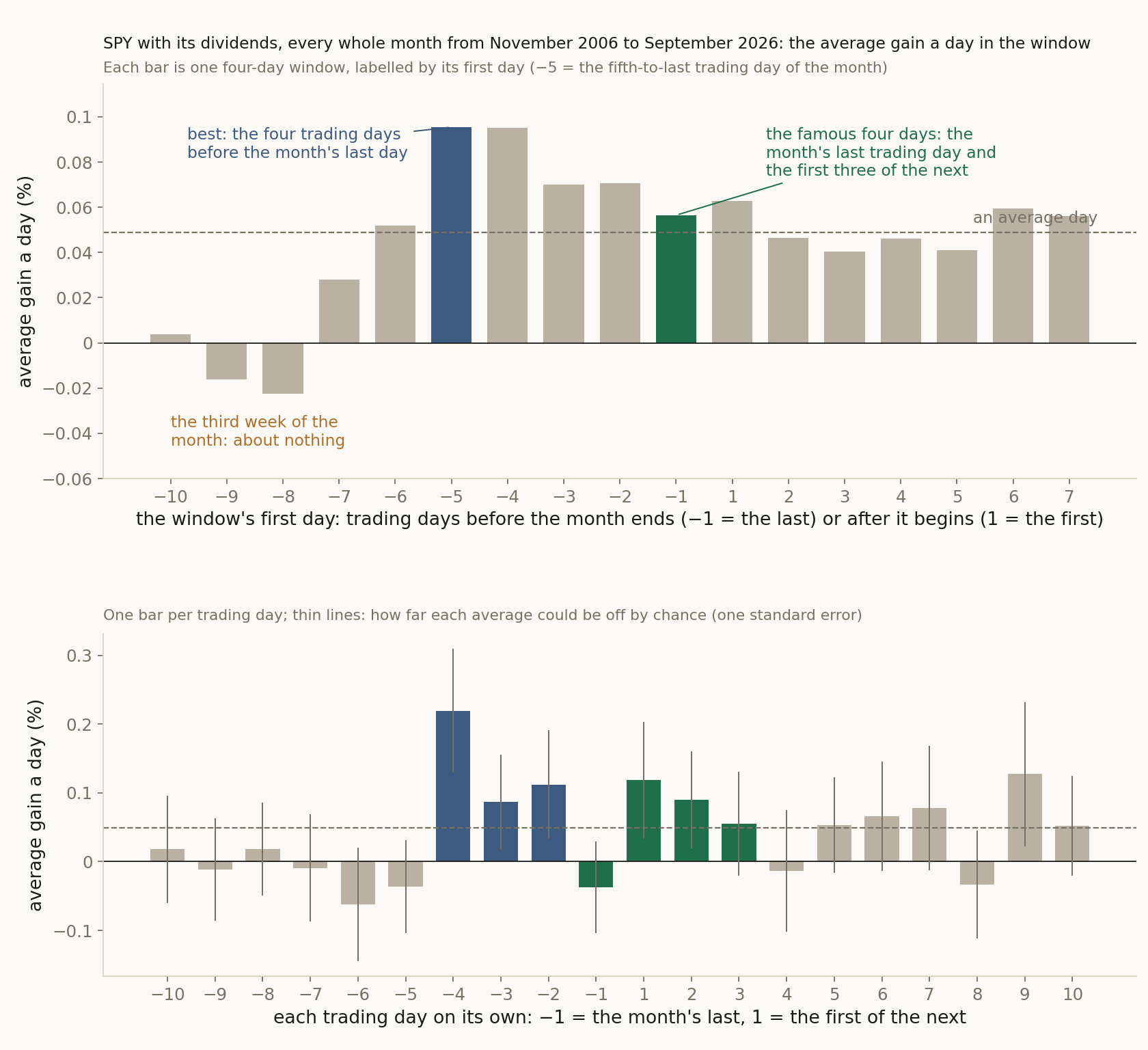
The famous window covers the last trading day of one month and the first three of the next. We kept the window four trading days long and slid it one day at a time, from ten trading days before the month ends to the seventh trading day of the next month. Owning a window means buying at the closing price of the day before its first day and selling at the closing price of its last day (Figure 5 shows it). At each stop we averaged SPY's daily gain in the window, dividends included, over every month from November 2006 to September 2026.

Figure 2 shows where the gain sits. The best stretch is the four trading days before the month's last day, which gained 0.095% a day, about twice an average day of 0.049%. The window one day later gained the same, because the day it drops and the day it adds, the fifth-to-last and the last trading day, both lost money on average. The famous window gained 0.057% a day, a little above an average day, and its first day is the reason: the month's last day lost money on average, while the first two days of the new month gained more than an average day. The windows in the third week of the month, from the tenth- to the fifth-to-last trading day, earned about nothing.

The single days in the bottom chart need care. Each day's average could be off by about 0.08% by chance, the thin lines, and on that scale only one day stands clear of an average day: the fourth-to-last trading day of the month. That is the day where Etula and his coauthors found the payday starting, long before we looked, so it is a test of their finding rather than our pick. The pattern they describe, funds selling to raise cash in the third week and prices recovering in the last days of the month, fits the rest of the chart.

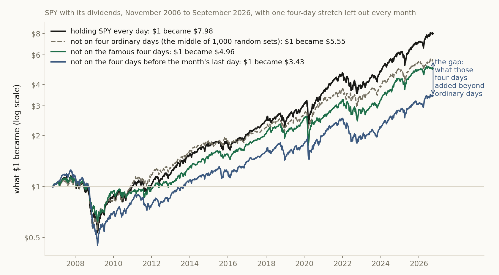
Figure 1 puts it in dollars, as the gap between holding SPY and holding it with one stretch left out. Held every day, $1 became $7.98 over the twenty years. Leaving out any four days a month costs a lot, because that is a fifth of the trading days: leaving out four ordinary days, the middle of 1,000 random sets, left $5.55. Leaving out the famous four days left $4.96, a deeper cut than about six in ten random sets, so close to ordinary days. Leaving out the four days before the month's last day left $3.43. That stretch is the best of seventeen windows, picked after looking, and the best of seventeen would cut that deep most of the time by luck alone, so the figure shows where the gain sat in these twenty years. The reason to believe in a payday is that Etula and his coauthors found it starting on the same day in US data back to 1926.

Traded over the locked tests from 2012 to 2026 on prices alone (Tables 4 and 5), the third-week windows lost money, partly because SPY's quarterly dividend comes out of the price in those days. The famous window came 10th of the 17 windows on SPY and 16th on IWM. The best window in those years, on both funds, was the fourth to seventh trading day of the new month, which the twenty-year averages put close to an average day, so which window wins depends on the years.

Stocks, bonds and gold

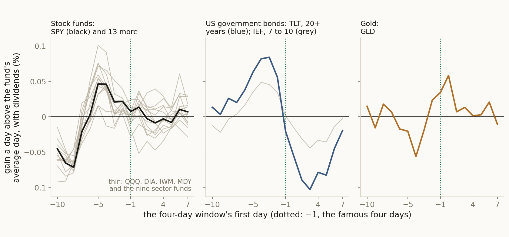
If the payday comes from funds raising cash and putting it back, it should show up across the stock market, not only in SPY. The left chart below repeats the slide for 14 stock funds: SPY, the Dow (DIA), the Nasdaq-100 (QQQ), mid-sized and small companies (MDY and IWM), and the nine sector funds. Every one has the same pattern: below its average day in the third week of the month, above it in the last days.

Bonds and gold are the control. US government bond funds (TLT, which holds bonds of more than 20 years, and IEF, of 7 to 10 years) rise in the last days of the month, a pattern of their own that Hartley and Schwarz (2019) found in Treasury bonds, and slip back in the first week of the next. Gold does not follow the stocks: its line wanders about as much, but with no dip in the third week and no rise in the last days of the month.

These charts describe twenty years. They were not fixed in advance, the funds overlap, and with seventeen windows to compare, one will stand out by chance. Against that, the pattern repeats in all 14 stock funds, gold does not have it, and Etula and his coauthors found it in US data back to 1926.

Bonus: skipping the third week

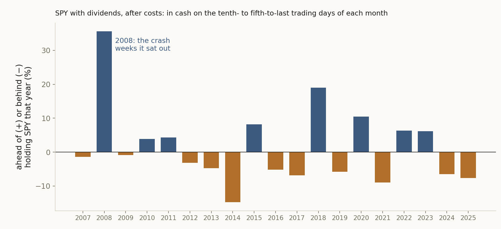
If the third week earns about nothing, holding SPY on every other day should beat holding it all the time. On prices alone it seems to. From 2012 to 2026, sitting in cash from the tenth- to the fifth-to-last trading day of each month and holding SPY the rest of the time ended at $5.96 after trading costs, against $5.76 for holding SPY.

But SPY's dividend comes out of its price in the third week of March, June, September and December, and an investor who is in cash that day does not receive it. With dividends counted, from 2012 to 2026 skipping the third week ended at $6.26, against $7.42 for holding SPY. Over the whole twenty years it came out ahead, but it beat holding in only 8 of the 19 full years from 2007 to 2025, and its lead rests on the crash weeks of 2008: without that year it would have ended 10% behind holding SPY. A backtest on prices alone would have shown the skip as a winner.

**Figure 3.** The same slide for 14 stock funds, for US government bonds and for gold, dividends included: the average gain a day in each four-day window above or below the fund's own average day, November 2006 to September 2026. The dotted line marks the famous four days.

**Figure 4.** Skipping the third week, year by year: how far a rule in cash on the tenth- to fifth-to-last trading days of each month, and in SPY the rest of the time, ended ahead of or behind holding SPY, dividends included, after trading costs, 2007 to 2025.

1 Methodology, in detail (click to open)

1 Methodology

The tests. Next we traded the payday, six months at a time, from January 2012 to July 2026: 29 tests in a row, each locked on the platform before it was scored, so no rule could be changed after a result. The rules were fixed before the first test, the famous four days exactly as Lakonishok and Smidt defined them in 1988. We had seen the twenty-year averages before the tests were locked, so the locking stops a rule from being changed; it cannot make the years unseen. The tests start in 2012 because one rule needs five whole years of months before its first test, and our data starts in October 2006.

The rules. The turn of the month: own SPY on the last trading day of the month and the first three of the next, buying at the closing price of the day before and selling at the closing price of the third day, and hold cash on the other days. The rest of the month: own SPY on all the other trading days. The best days of the last five years: each month, own SPY on the four days of the month (by their place in it) that paid best over the previous five years, using only months that had ended; a second test does the same with the last three years. Holding SPY: buy at the start of each test and hold to its end, with no trading cost.

Prices are daily closing prices from a licensed commercial data provider, without dividends, for the rules and for holding alike. Each purchase and each sale costs 0.02%, and cash earns nothing. The same tests ran on IWM, the Russell 2000 fund of small US companies.

Where a test starts. Each test starts in cash at the closing price of its first trading day, so the tests leave out 19 days: the first trading day of every January, and of July in the four years when 1 July fell on a weekend. All are turn of the month days. Counted in, the turn of the month would have turned $1 into $1.46 before costs on SPY, beating 61% of the random sets before costs and 82% after. The conclusions do not change.

The placebo. As with the sugar pill in a medical trial, each rule is compared with days chosen at random: four days of the month drawn at random once a year, in 1,000 random sets, each run over the same tests with the same trading cost. If a rule's days are special, it should beat nearly all of them. Five of the random sets also ran through the platform's own six-month test and matched it to the cent. Tables 4 and 5, which run every four-day window as a rule over the same tests, were added after the tests ran.

2 Results

2.1 Headline

The turn of the month, Sharpe

0.30

day by day, every year the test ran, 2012 to 2026

The rest of the month, Sharpe

0.69

day by day, every year the test ran, 2012 to 2026

The result

Over twenty years, $1 in SPY with its dividends became $7.98. Leaving out four ordinary days each month would have left about $5.55, the famous four days $4.96, and the four trading days before the month's last day $3.43.

**Figure 5.** How each rule trades: the trading days around the end of the month, with the days each rule holds SPY shaded, a purchase at the closing price before the first held day and a sale at the closing price of the last one.

**Figure 6.** What $1 became, January 2012 to July 2026, day by day: holding each fund, the turn of the month, the rest of the month and the best days of the last five (and three) years. Prices without dividends, 0.02% a purchase or a sale, cash earns nothing. The scale is logarithmic: equal steps up the side are equal percentage gains.

**Figure 7.** Did anything beat holding? Each bar counts the random sets of four days a month that ended at that value, out of 1,000, January 2012 to July 2026, after trading costs. The lines: the rules we tested, the rest of the month and holding the fund.

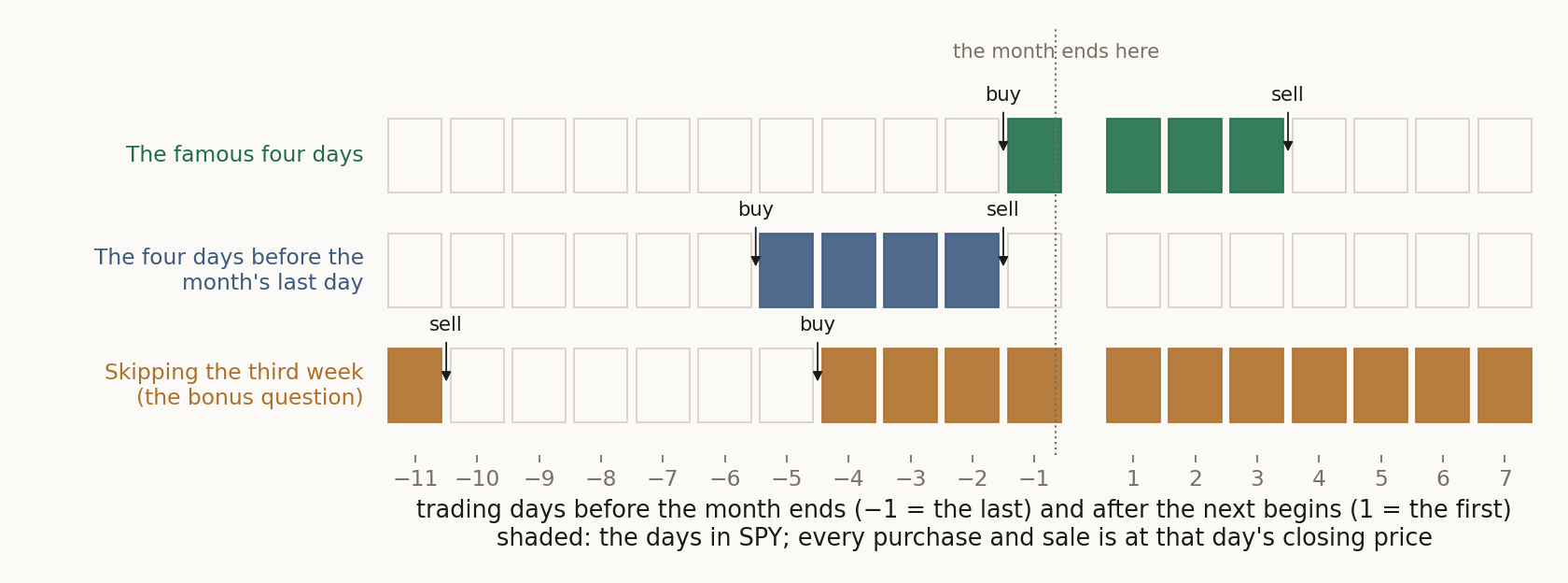
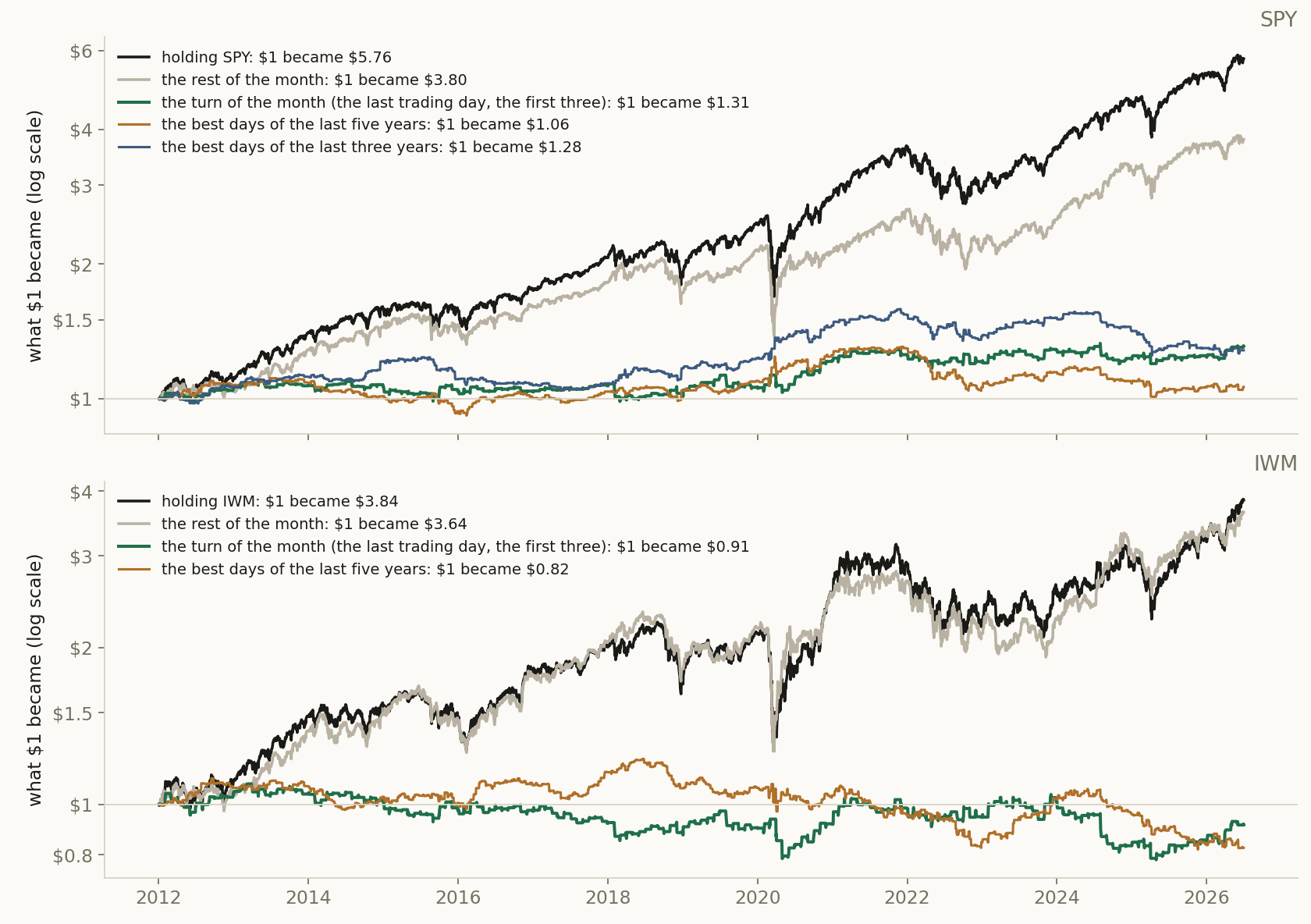
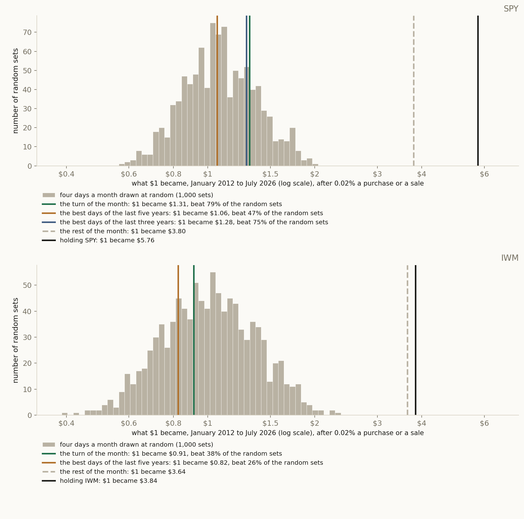
Table 1. What $1 became on SPY, January 2012 to July 2026. 29 six-month tests, each locked before it was scored (this page shows the record of the turn of the month against the rest; the records of the other tests are kept on the platform). SPY prices without dividends, 0.02% a purchase or a sale. Before costs the turn of the month ($1.41) and the rest of the month ($4.07) multiply back to holding ($5.76).

Rule	$1 became	A year	Worst fall	Time in SPY	Trades a year
Holding SPY	$5.76	12.8%	−34.1%	100%
A fifth of SPY, the rest in cash	$1.43	2.5%	−7.0%	a fifth, always
The rest of the month	$3.80	9.6%	−37.4%	81%	12
The turn of the month	$1.31	1.9%	−10.0%	19%	14
The best days of the last five years	$1.06	0.4%	−22.7%	19%	42
The best days of the last three years	$1.28	1.7%	−21.3%	19%	40

Table 2. What $1 became on IWM, small companies, January 2012 to July 2026. The same tests on IWM, the Russell 2000 fund; counted as in the first table.

Rule	$1 became	A year	Worst fall	Time in IWM	Trades a year
Holding IWM	$3.84	9.7%	−42.6%	100%
A fifth of IWM, the rest in cash	$1.35	2.1%	−9.1%	a fifth, always
The rest of the month	$3.64	9.3%	−46.1%	81%	12
The turn of the month	$0.91	−0.6%	−28.5%	19%	14
The best days of the last five years	$0.82	−1.3%	−33.0%	19%	41

Table 3. The rules against 1,000 sets of four random days. Each random set holds four days of the month (by place), drawn once a year, over the same 29 tests. Beat: the share of the random sets that ended lower. A random set buys about 41 times a year, the turn of the month 14, and each purchase is later sold.

Rule	Fund	After costs: $1 became	Beat	Before costs: $1 became	Beat
The turn of the month	SPY	$1.31	79%	$1.41	58%
The best days of the last five years	SPY	$1.06	47%	$1.35	49%
The best days of the last three years	SPY	$1.28	75%	$1.61	74%
The middle random set	SPY	$1.07	50%	$1.36	50%
The turn of the month	IWM	$0.91	38%	$0.98	21%
The best days of the last five years	IWM	$0.82	26%	$1.04	26%
The middle random set	IWM	$1.01	50%	$1.28	50%

Table 4. The sliding window, part one: windows starting in the old month. −1 is the last trading day of the month, 1 the first of the next. Average a day: SPY with dividends, every whole month from November 2006 to September 2026. $1 became: owning the fund only in that window over the 29 tests, January 2012 to July 2026, prices without dividends, before trading costs.

Window	SPY: average a day	SPY: $1 became	IWM: $1 became
−10 to −7	0.004%	$0.92	$1.05
−9 to −6	−0.016%	$0.86	$0.99
−8 to −5	−0.022%	$0.87	$1.00
−7 to −4	0.028%	$1.16	$1.31
−6 to −3	0.052%	$1.29	$1.43
−5 to −2	0.095%	$1.75	$1.86
−4 to −1	0.095%	$1.61	$1.33
−3 to 1	0.070%	$1.60	$1.29
−2 to 2	0.071%	$1.67	$1.34
−1 to 3 (the famous four days)	0.057%	$1.41	$0.98

Table 5. The sliding window, part two: windows starting in the new month. Counted as in Table 4.

Window	SPY: average a day	SPY: $1 became	IWM: $1 became
1 to 4	0.063%	$1.69	$1.33
2 to 5	0.046%	$1.62	$1.39
3 to 6	0.040%	$1.61	$1.51
4 to 7	0.046%	$1.90	$1.98
5 to 8	0.041%	$1.56	$1.38
6 to 9	0.059%	$1.31	$1.11
7 to 10	0.056%	$1.37	$0.97

Sections 2.2 to 3, the full record: every year, every test, and how each one was run (click to open)

2.2 Per-step results

**Table 6.** One row per step, raw out-of-sample results. A short window can pair a negative return with a positive annualised Sharpe: at high daily volatility the arithmetic mean of daily returns sits above the compounded window return, and the Sharpe reads the former. Volatility drag, printed rather than smoothed.
#	Out-of-sample window	The turn of the month SR	The rest of the month SR
1	2012-01-03 → 2012-06-29	0.45	0.89
2	2012-07-02 → 2012-12-31	1.71	-0.12
3	2013-01-02 → 2013-07-01	0.12	1.82
4	2013-07-01 → 2013-12-31	0.62	2.63
5	2014-01-02 → 2014-07-01	0.58	1.26
6	2014-07-01 → 2014-12-31	-0.79	1.13
7	2015-01-02 → 2015-07-01	-0.94	0.68
8	2015-07-01 → 2015-12-31	0.12	-0.22
9	2016-01-04 → 2016-07-01	0.53	0.37
10	2016-07-01 → 2016-12-30	-1.19	1.79
11	2017-01-03 → 2017-06-30	1.47	1.43
12	2017-07-03 → 2017-12-29	0.80	2.91
13	2018-01-02 → 2018-06-29	-1.22	0.95
14	2018-07-02 → 2018-12-31	0.88	-1.29
15	2019-01-02 → 2019-07-01	1.97	1.81
16	2019-07-01 → 2019-12-31	-1.41	2.56
17	2020-01-02 → 2020-07-01	0.54	-0.18
18	2020-07-01 → 2020-12-31	2.50	1.14
19	2021-01-04 → 2021-07-01	1.30	1.94
20	2021-07-01 → 2021-12-31	-0.48	1.96
21	2022-01-03 → 2022-07-01	-0.69	-1.59
22	2022-07-01 → 2022-12-30	0.13	0.05
23	2023-01-03 → 2023-06-30	2.08	1.33
24	2023-07-03 → 2023-12-29	-0.09	1.33
25	2024-01-02 → 2024-07-01	0.29	2.96
26	2024-07-01 → 2024-12-31	-1.37	2.11
27	2025-01-02 → 2025-07-01	0.20	0.48
28	2025-07-01 → 2025-12-31	0.18	1.90
29	2026-01-02 → 2026-07-01	2.10	0.46

Figure 8. The turn of the month: every step's out-of-sample curve overlaid, each rebased to 1× at its own start. Read alongside the per-step table: consistent shape across steps is the walk-forward's evidence; a single lucky leg is not.

Figure 9. The rest of the month: the same windows, the other arm. Compare shape-for-shape with the previous figure: the two arms trade the identical out-of-sample windows.

2.3 Search accounting

No search record exists for this design. It was not promoted from a recorded evolving search, so the number of alternatives tried before it, on paper, in another tool, or in the author's head, is unknown. Unknown is a different fact from one: a study with no lineage is not a strategy with one trial, it is a strategy with an unrecorded number of them. Accordingly no count of alternatives tried is claimed, and nothing in this paper is corrected for a search that was never recorded; the number that stands is the raw out-of-sample result plus this disclosure. The registered per-step record below (§4) still guarantees each window's hypothesis was hashed and registered before that window was scored.

2.4 The comparison

Both arms trade the same registered windows, so their returns can be PAIRED: inside each window the two return series are inner-joined date by date and the difference r_{The turn of the month} − r_{The rest of the month} is the object under test. Because this is ONE pre-declared contrast, frozen at registration before any window was scored, the paired statistic needs no multiple-testing deflation, and the per-arm pooled numbers above are likewise uncorrected, because this design has no recorded search to correct against (§2.3). The paired contrast carries that gap differently from the arm levels: it was declared before each window ran and it is scored on the difference, so no window could be read first and scored after. What the timestamps cannot speak to is how this contrast came to be the declared one, which is the limit §2.3 states.

In the table: Arm A = The turn of the month · Arm B = The rest of the month.

**Table 7.** Window-by-window paired comparison. Δ is the growth gap (Arm A − Arm B) over the window's paired dates.
#	Window	Paired bars	Arm A	Arm B	Δ	Leader
1	2012-01-04 → 2012-06-29	124	+1.3%	+4.9%	-3.6 pp	Arm B
2	2012-07-03 → 2012-12-31	124	+4.8%	-0.9%	+5.7 pp	Arm A
3	2013-01-03 → 2013-07-01	124	+0.2%	+9.7%	-9.4 pp	Arm B
4	2013-07-02 → 2013-12-31	127	+1.0%	+12.8%	-11.9 pp	Arm B
5	2014-01-03 → 2014-07-01	124	+1.3%	+5.8%	-4.6 pp	Arm B
6	2014-07-02 → 2014-12-31	127	-2.1%	+6.0%	-8.1 pp	Arm B
7	2015-01-05 → 2015-07-01	124	-2.7%	+3.4%	-6.1 pp	Arm B
8	2015-07-02 → 2015-12-31	127	+0.3%	-2.5%	+2.8 pp	Arm A
9	2016-01-05 → 2016-07-01	125	+1.7%	+2.2%	-0.5 pp	Arm B
10	2016-07-05 → 2016-12-30	126	-1.8%	+7.9%	-9.8 pp	Arm B
11	2017-01-04 → 2017-06-30	124	+2.2%	+4.6%	-2.4 pp	Arm B
12	2017-07-05 → 2017-12-29	125	+1.0%	+8.5%	-7.5 pp	Arm B
13	2018-01-03 → 2018-06-29	124	-5.4%	+6.2%	-11.6 pp	Arm B
14	2018-07-03 → 2018-12-31	125	+2.6%	-10.8%	+13.4 pp	Arm A
15	2019-01-03 → 2019-07-01	124	+7.8%	+9.1%	-1.3 pp	Arm B
16	2019-07-02 → 2019-12-31	127	-4.9%	+13.9%	-18.7 pp	Arm B
17	2020-01-03 → 2020-07-01	125	+3.3%	-7.9%	+11.2 pp	Arm A
18	2020-07-02 → 2020-12-31	127	+11.0%	+8.0%	+3.0 pp	Arm A
19	2021-01-05 → 2021-07-01	124	+4.3%	+11.3%	-7.0 pp	Arm B
20	2021-07-02 → 2021-12-31	127	-1.5%	+11.4%	-12.9 pp	Arm B
21	2022-01-04 → 2022-07-01	124	-3.9%	-17.4%	+13.5 pp	Arm A
22	2022-07-05 → 2022-12-30	126	+0.4%	-0.6%	+1.0 pp	Arm A
23	2023-01-04 → 2023-06-30	123	+6.8%	+8.5%	-1.7 pp	Arm B
24	2023-07-05 → 2023-12-29	125	-0.3%	+6.9%	-7.2 pp	Arm B
25	2024-01-03 → 2024-07-01	124	+0.8%	+14.0%	-13.2 pp	Arm B
26	2024-07-02 → 2024-12-31	127	-5.3%	+13.0%	-18.3 pp	Arm B
27	2025-01-03 → 2025-07-01	122	+0.7%	+4.4%	-3.7 pp	Arm B
28	2025-07-02 → 2025-12-31	127	+0.4%	+9.5%	-9.1 pp	Arm B
29	2026-01-05 → 2026-07-01	123	+5.9%	+2.6%	+3.3 pp	Arm A

Paired Sharpe of the difference track: -0.50 · block bootstrap (2000 paths, block 10, seed 1234): P(The turn of the month beats The rest of the month) = 3.9%.

Window win-rate. The turn of the month led 8 of 29 windows (27.6%), The rest of the month led 21, and the mean window gap of -3.95 pp points the same way. Widest single window: 2019 at -18.7 pp.

3 The circuit

The strategy is a circuit of platform primitives, frozen when the study is registered. Below is the circuit as wired on the canvas, the objective it encodes and how the search runs through it, followed by the mathematics each primitive actually computes, the same formulas the execution engine runs. The complete parameterisation is preserved in the study ledger (Appendix A).

The hypothesis under test

The sentence below is the registered design with its rules in plain words; the exact registration record is in Appendix A2; the authored description of the design is Section 1.

A COMPARATIVE study: The turn of the month vs The rest of the month, walked on the same registered out-of-sample windows. The turn of the month: SPY, bought when the next session is one of the last session of the month and the first three of the next; sell when the next session is not one of the last session of the month and the first three of the next, and forward-tested out-of-sample from the anchor: the rule set is frozen at the anchor, with no in-sample re-optimization. The rest of the month: SPY, bought when the next session is not one of the last session of the month and the first three of the next; sell when the next session is one of the last session of the month and the first three of the next, and forward-tested out-of-sample from the anchor: the rule set is frozen at the anchor, with no in-sample re-optimization. The arms differ in: Signal Module, config (entry · operator: above → below; exit · operator: below → above). The contrast under test: whether The turn of the month generates better risk-adjusted returns than The rest of the month over the identical out-of-sample windows.

Every block in this study is a card from the platform's catalog: SPY and its price loader, the signal module that uses the Day of the Month indicator, the six-month test and the trading cost. The Day of the Month indicators give each trading day its place in the month: fixed days, learned days and random days for a placebo, so a reader can rebuild every test.

Figure 10. The frozen circuit, every node a primitive, every wire a typed data-flow; the two arms are colour-coded (The turn of the month green, The rest of the month blue, shared feeds neutral). Each box is one step of the strategy; data flows along the wires left to right, and no box can see data dated later than the box feeding it. The whole diagram was frozen when the hypothesis was registered. Click any node to open what that step ran with and what it produced.

Envelopes show counts, ratios, dates, and the parameters the author chose. Full price and per-name data series are not republished: the underlying market data is licensed to QuanterLab. Point figures quoted in the prose, a named holding's return over a stated span, are summary facts derived from public market prices, not redistributed series.

What each part does

Ticker, A single instrument symbol, the seed of a single-name circuit.

Ticker Price Loader, Single-ticker OHLCV loader, the deep window a signal needs.

Signal Module, The entry / exit rule, turn indicators into a per-bar trade signal.

Backtest Validator, Forward-test the winning rule on unseen, out-of-sample data.

Transaction Cost, Charge for trading, slippage + commission on every turn.

The objective and the search

The turn of the month

Universe	Single ticker SPY with 365 days (~1.0y) of price history.
Signal generation	buy when the next session is one of the last session of the month and the first three of the next; sell when the next session is not one of the last session of the month and the first three of the next.
Validation & out-of-sample	signal forward test (6m horizon from the anchor); overlays: Transaction Cost.

The rest of the month

Signal generation	buy when the next session is not one of the last session of the month and the first three of the next; sell when the next session is one of the last session of the month and the first three of the next.

Every other specification row is identical to The turn of the month's table above.

What differs between the arms, one difference; the comparison is clean:

paramSignal Module, config
- · buy when: the next session is one of the last session of the month and the first three of the next (The turn of the month); the next session is not one of the last session of the month and the first three of the next (The rest of the month)
- · sell when: the next session is not one of the last session of the month and the first three of the next (The turn of the month); the next session is one of the last session of the month and the first three of the next (The rest of the month)

Everything else is held identical, so an out-of-sample gap between the arms is attributable to this one change.

Cost elements are wired into the circuit.

Show the mathematics, 5 primitives, formulas and parity notes

3.1 Ticker

A single instrument symbol, the seed of a single-name circuit.

No math. It just names one stock and hands the symbol to a Ticker Price Loader, which fetches its price history.

What it is

A constant: one ticker string. The computation lives downstream in the loader and the signal.

3.2 Ticker Price Loader

Single-ticker OHLCV loader, the deep window a signal needs.

Same as the bulk loader but for one name, fetching a deep lifecycle window so an indicator or stochastic signal has enough history to warm up.

What it loads

One ticker's OHLCV up to the anchor, length set by the strategy's warm-up requirement.

P = \{(o,h,l,c,v)_\tau : \tau \le t\}

3.3 Signal Module

The entry / exit rule, turn indicators into a per-bar trade signal.

Composes indicators (RSI, moving averages, …) with comparison and logic operators into a rule that says enter, exit, or hold each bar. The rule is emitted as a portable config the optimizer tunes and the walk-forward validates, so what you design is exactly what gets traded.

Boolean rule → position state

\text{signal}_t = \begin{cases} +1 & \text{entry rule true} \\ 0 & \text{exit rule true} \\ \text{hold} & \text{otherwise}\end{cases}

e.g. enter when RSI < 30, exit when RSI > 50.

3.4 Backtest Validator

Forward-test the winning rule on unseen, out-of-sample data.

Takes the wired rule config (the Walk-Forward validated config wins, else the optimized config, else the raw signal config) and trades it FORWARD on the out-of-sample window to the right of the anchor, data it never saw during optimization, re-deriving the regime as-of each bar. It produces the true out-of-sample equity curve, trades and statistics: the signal-path twin of the Portfolio Forward Test, not an in-sample replay.

Apply the frozen rule forward (OOS)

E_t = E_{t-1}\,(1 + r_t),\qquad \text{Sharpe} = \frac{\bar r - r_f}{\sigma_r}\sqrt{252}

Config frozen from optimization / walk-forward, then replayed bar-by-bar on the forward window it has never seen, with cost + risk overlays applied.

3.5 Transaction Cost

Charge for trading, slippage + commission on every turn.

Real trading isn't free. This deducts a cost proportional to how much you trade (turnover), in basis points, so the backtest reflects net, not gross, performance.

Cost per rebalance

\text{cost}_t = \frac{\text{bps}}{10{,}000}\;\times\;\text{turnover}_t, \qquad \text{turnover}_t = \tfrac12\sum_i \lvert w_{i,t}-w_{i,t^-}\rvert

4 Discussion

4.1 Findings

The answer. Owning SPY at the turn of the month turned $1 into $1.31 from 2012 to 2026, owning it on all the other days $3.80, and holding SPY $5.76.

No rule beat holding SPY, and on IWM no rule beat holding IWM.

The famous four days became ordinary. They were in the market a fifth of the time, and keeping a fifth of the money in SPY all the time, with the rest in cash, did about as well: $1.43 against their $1.41 before trading costs. Owning SPY only in the last four trading days of the month did better than that yardstick, $1.61 before costs, though that is a window we picked after seeing the averages, so it stays a description.

On small companies the famous four days did worse: on IWM they ended at $0.91 after costs, holding IWM at $3.84, and only one of the 17 four-day windows in Tables 4 and 5 did worse than them.

The placebo. Four random days are rarely next to each other, so a random set buys and sells about three times as often as the turn of the month and pays about three times as much in trading costs. After costs, the turn of the month beat 79% of the random sets on SPY. Before costs it beat 58%, about as well as days picked at random. On IWM, four in five random sets did better than it, before costs.

Following the payday. The best days of the last five years ended at $1.06 on SPY and beat 47% of the random sets, what luck alone would give. With a three-year memory the rule did better before costs, but it traded about three times as often and ended just behind the turn of the month after costs, at $1.28.

None of the rules reached the best tenth of the random sets: each result is one that luck alone could produce. The tests rule out the old pattern, in which the four days carried all of the gain; they cannot rule out that a day at the turn of the month earns up to about 0.09% more than an ordinary day.

4.2 Interpretation

Where the payday went. It did not go far. It sits in the last days of the month, where Etula and his coauthors found it, and the famous four days start on the month's last day, which lost money on average. That is why tests of the famous window find so little. Stocks across the market show it, and gold does not. That fits a payday made by the cash that funds raise and put back at the month's end.

The rules of trading may move it a little. While US trades settled in three days, until 2017, the strongest days were the fourth- and third-to-last; once they settled in two days, the strongest was the second-to-last. That is the direction a payday tied to settlement should move, but each of these averages could be off by about 0.13% by chance, so it is a hint. We had expected the payday to move earlier, as buyers tried to get ahead of it, and the data do not show that.

A rule that chases the best days of the past picked days no better than chance. For someone who holds the S&P 500, nothing here beat staying in SPY.

Others have studied the money that moves around the month, and we credit their work here without testing it. Concretum Research (2026) trades SPY against TLT ahead of month-end rebalancing. Ma and Pratt (2018) found a second payday in the middle of the month, on the 16th. Nathan, Suominen and Tasa (2026) found that the extra gain of recent winners over recent losers (momentum) comes mostly on six trading days before the month ends. Hartzmark and Solomon (2025) found that the market tends to rise on the days large dividends are paid out.

Three questions stay open. The last days of the month deserve their own test, locked before it runs. One-day settlement, since May 2024, should move the payday again, and two years of months are too few to see it. And other markets may differ. This study's test opens in the lab, where each rule is one click away.

Enter the lab

Press Open the platform and this study's test opens in the lab, our research workspace: SPY and its prices, the turn of the month and the rest of the month side by side, the six-month test and the trading cost. The three Day of the Month indicators are in the indicator list: fixed days, learned days and random days, the placebo.

Things to try. Slide the window yourself: set the fixed days to the last four trading days of the month and none of the next. Give the learned days a one-year memory. Change the fund. Or draw a new set of random days.

4.3 Limitations

The sliding charts and the bonus question count dividends. The locked tests, the random sets and the four-day windows run as trades use prices without dividends, for the rules and for holding alike; none of those rules holds SPY on its dividend days any more than random days do, but a rule that skips the third week does, and the bonus question shows how much that matters. Cash earns nothing here; interest would help the rules, which are in cash most of the time, most of all from 2022, when rates rose. There is one trading cost, 0.02% a purchase or a sale, on the high side for SPY; the before-costs results show the other end. The sliding averages, the comparison of funds and the bonus question describe twenty years; they were not locked in advance.

References

QuanterLab reference architecture

Gelman, A., & Loken, E. (2013). The garden of forking paths: Why multiple comparisons can be a problem, even when there is no “fishing expedition.” Working paper, Columbia University.
Harvey, C. R., Liu, Y., & Zhu, H. (2016). … and the Cross-Section of Expected Returns. Review of Financial Studies, 29(1), 5–68. doi:10.1093/rfs/hhv059
Lo, A. W. (2002). The Statistics of Sharpe Ratios. Financial Analysts Journal, 58(4), 36–52. doi:10.2469/faj.v58.n4.2453

Author’s references?

Ariel (1987), A Monthly Effect in Stock Returns, Journal of Financial Economics 18(1): from 1963 to 1981 the US market's gain came in the first half of the month. https://doi.org/10.1016/0304-405X(87)90066-3
Lakonishok and Smidt (1988), Are Seasonal Anomalies Real? A Ninety-Year Perspective, Review of Financial Studies 1(4): the last trading day of the month and the first three of the next, in ninety years of the Dow. https://doi.org/10.1093/rfs/1.4.403
Ogden (1990), Turn-of-Month Evaluations of Liquid Profits and Stock Returns: A Common Explanation for the Monthly and January Effects, Journal of Finance 45(4): payments made at the turn of the month and the gains that follow them. https://doi.org/10.1111/j.1540-6261.1990.tb02435.x
McConnell and Xu (2008), Equity Returns at the Turn of the Month, Financial Analysts Journal 64(2): from 1926 to 2005 US investors were paid for market risk only at the turn of the month; the pattern appears in 31 of 35 countries. https://doi.org/10.2469/faj.v64.n2.11
Etula, Rinne, Suominen and Vaittinen (2020), Dash for Cash: Monthly Market Impact of Institutional Liquidity Needs, Review of Financial Studies 33(1): month-end cash needs move prices; since 1926 the US excess return came in the seven days from the fourth-to-last trading day to the third of the next. https://doi.org/10.1093/rfs/hhz054
Hartley and Schwarz (2019), Predictable End-of-Month Treasury Returns, SSRN working paper: Treasury bonds tend to rise in the last days of the month. https://doi.org/10.2139/ssrn.3440417
Hartzmark and Solomon (2025), Market-Wide Predictable Price Pressure, American Economic Review 115(9): the market tends to rise on days large dividends are paid. https://doi.org/10.1257/aer.20231725
Harvey, Mazzoleni and Melone (2025), The Unintended Consequences of Rebalancing, NBER Working Paper 33554: funds that rebalance stocks and bonds on the calendar move prices. https://doi.org/10.2139/ssrn.5122748
Nathan, Suominen and Tasa (2026), The Intramonth Momentum Cycle, SSRN working paper (Quantpedia Awards 2026): month-end selling, and the day it moved with next-day settlement in 2024. https://doi.org/10.2139/ssrn.6426026
Ma and Pratt (2018), Payday Anomaly, SSRN working paper: a second payday in the middle of the month, on the 16th. https://ssrn.com/abstract=3257064
Concretum Research (2026), How to Generate Alpha From Rebalancing Flows: trading SPY against TLT ahead of month-end rebalancing. https://concretumgroup.substack.com/p/how-to-generate-alpha-from-rebalancing

Appendix A Reproducibility in QuanterLab

Each step is backed by a frozen run report. The study is re-derivable from the ledger below.

#	Commit	Report	Anchor	OOS window
1	ae225e547c8c	13675	2012-01-01	2012-01-03 → 2012-06-29
2	c731c8019ed5	13676	2012-07-01	2012-07-02 → 2012-12-31
3	e354043aa83c	13677	2013-01-01	2013-01-02 → 2013-07-01
4	d20de0bdce3f	13678	2013-07-01	2013-07-01 → 2013-12-31
5	ed32764cfc2b	13679	2014-01-01	2014-01-02 → 2014-07-01
6	cb10d3b87d44	13680	2014-07-01	2014-07-01 → 2014-12-31
7	0070328e7072	13681	2015-01-01	2015-01-02 → 2015-07-01
8	70c34b4af21d	13682	2015-07-01	2015-07-01 → 2015-12-31
9	2e9a9b1896fa	13683	2016-01-01	2016-01-04 → 2016-07-01
10	845db43c343a	13684	2016-07-01	2016-07-01 → 2016-12-30
11	3f98b8723edb	13685	2017-01-01	2017-01-03 → 2017-06-30
12	b6eec34a647f	13686	2017-07-01	2017-07-03 → 2017-12-29
13	00e92b357e69	13687	2018-01-01	2018-01-02 → 2018-06-29
14	8fe43d610bb9	13688	2018-07-01	2018-07-02 → 2018-12-31
15	2a263ea3d7c1	13689	2019-01-01	2019-01-02 → 2019-07-01
16	8ff96dfcb9de	13690	2019-07-01	2019-07-01 → 2019-12-31
17	1b4d4433f253	13691	2020-01-01	2020-01-02 → 2020-07-01
18	63e2ee672b17	13692	2020-07-01	2020-07-01 → 2020-12-31
19	5e611aee2786	13693	2021-01-01	2021-01-04 → 2021-07-01
20	74f9801c5d57	13694	2021-07-01	2021-07-01 → 2021-12-31
21	7e5674d33a10	13695	2022-01-01	2022-01-03 → 2022-07-01
22	100a0310b73e	13696	2022-07-01	2022-07-01 → 2022-12-30
23	8f22e5728c1a	13697	2023-01-01	2023-01-03 → 2023-06-30
24	c85b8c7d08d4	13698	2023-07-01	2023-07-03 → 2023-12-29
25	a4c23d7fd889	13699	2024-01-01	2024-01-02 → 2024-07-01
26	48dc732f27ba	13700	2024-07-01	2024-07-01 → 2024-12-31
27	1cfe37176b51	13701	2025-01-01	2025-01-02 → 2025-07-01
28	e650f5b3f542	13702	2025-07-01	2025-07-01 → 2025-12-31
29	8f2569d0bebd	13703	2026-01-01	2026-01-02 → 2026-07-01

Appendix A2 Registration record

What this record does and does not establish. Every window in this study is historical: the data existed before the study began, so this is sequential registration on past windows, not pre-registration in the clinical-trial sense, and no procedure could make it so. What the platform does enforce is order, each step's specification was frozen and hashed before that step was scored, and the walk cannot advance past a step that was never run or close one with a result registered for a different window. The two timestamp columns below are the evidence: read them together and each registration precedes its own run, and each run precedes the next registration. A study whose registrations all post-date its runs would show it here. Wall-clock spacing between registrations varies with the author's schedule and queue latency; the ordering, not the tempo, is the claim.

“A COMPARATIVE study: The turn of the month vs The rest of the month, walked on the same registered out-of-sample windows. The turn of the month: SPY, bought when the next session is one of the last session of the month and the first three of the next; sell when the next session is not one of the last session of the month and the first three of the next, and forward-tested out-of-sample from the anchor: the rule set is frozen at the anchor, with no in-sample re-optimization. The rest of the month: SPY, bought when the next session is not one of the last session of the month and the first three of the next; sell when the next session is one of the last session of the month and the first three of the next, and forward-tested out-of-sample from the anchor: the rule set is frozen at the anchor, with no in-sample re-optimization. The arms differ in: Signal Module, config (entry · operator: above → below; exit · operator: below → above). The contrast under test: whether The turn of the month generates better risk-adjusted returns than The rest of the month over the identical out-of-sample windows.”

The same hypothesis was registered independently at every step, hashed before each step's out-of-sample window was scored:

**Table 8.** Registration audit, one row per registered step, with the time each specification was frozen and the time its window was scored. The hypothesis is identical on every row by design: it was registered once and re-registered unchanged at each anchor. Rows that differ would mean the specification moved mid-walk, which is the thing this record exists to rule out. The timestamps are the separate claim: each registration precedes its own run, and each run precedes the next registration.
#	Anchor	Registered at (UTC)	Run completed (UTC)
1	2012-01-01	2026-10-03 13:36:20	2026-10-03 13:36:21
2	2012-07-01	2026-10-03 13:36:21	2026-10-03 13:36:22
3	2013-01-01	2026-10-03 13:36:22	2026-10-03 13:36:23
4	2013-07-01	2026-10-03 13:36:23	2026-10-03 13:36:25
5	2014-01-01	2026-10-03 13:36:25	2026-10-03 13:36:26
6	2014-07-01	2026-10-03 13:36:26	2026-10-03 13:36:27
7	2015-01-01	2026-10-03 13:36:27	2026-10-03 13:36:28
8	2015-07-01	2026-10-03 13:36:28	2026-10-03 13:36:29
9	2016-01-01	2026-10-03 13:36:29	2026-10-03 13:36:30
10	2016-07-01	2026-10-03 13:36:30	2026-10-03 13:36:31
11	2017-01-01	2026-10-03 13:36:31	2026-10-03 13:36:33
12	2017-07-01	2026-10-03 13:36:33	2026-10-03 13:36:34
13	2018-01-01	2026-10-03 13:36:34	2026-10-03 13:36:35
14	2018-07-01	2026-10-03 13:36:35	2026-10-03 13:36:36
15	2019-01-01	2026-10-03 13:36:36	2026-10-03 13:36:37
16	2019-07-01	2026-10-03 13:36:37	2026-10-03 13:36:38
17	2020-01-01	2026-10-03 13:36:38	2026-10-03 13:36:39
18	2020-07-01	2026-10-03 13:36:39	2026-10-03 13:36:40
19	2021-01-01	2026-10-03 13:36:40	2026-10-03 13:36:42
20	2021-07-01	2026-10-03 13:36:42	2026-10-03 13:36:43
21	2022-01-01	2026-10-03 13:36:43	2026-10-03 13:36:44
22	2022-07-01	2026-10-03 13:36:44	2026-10-03 13:36:45
23	2023-01-01	2026-10-03 13:36:45	2026-10-03 13:36:46
24	2023-07-01	2026-10-03 13:36:46	2026-10-03 13:36:47
25	2024-01-01	2026-10-03 13:36:47	2026-10-03 13:36:48
26	2024-07-01	2026-10-03 13:36:48	2026-10-03 13:36:49
27	2025-01-01	2026-10-03 13:36:49	2026-10-03 13:36:51
28	2025-07-01	2026-10-03 13:36:51	2026-10-03 13:36:52
29	2026-01-01	2026-10-03 13:36:52	2026-10-03 13:36:53