QuanterLab · Research

A Stochastic Model Against a Geometric Rule: the Kalman Filter and the 200-Day Line

The 200-day line draws the trend on the chart; a Kalman filter estimates it as a path hidden in noisy prices. Given the same horizon and walked a year at a time, the filter left the market less than a third as often on fourteen funds and ended ahead on SPY.

By Serhat Girgin

How this study was run: the companies, the method, the dates

Universe · S&P 500 (membership resolution not recorded)

Method · Comparative: Kalman filter vs 200-day line

Manipulated variable ·

Two arms trade the S&P 500 fund (SPY) from each first of January for a year, with the whole book in the fund or in cash. Arm B, the 200-day switch, holds the fund while its close is above its 200-day average and sells to cash at the first close below it; it buys back at the first close above. Arm A, the Kalman switch, reads the same closes through the Kalman Trend card, a filter that keeps a running estimate of the price level and of its slope; it holds the fund while the slope points up and sells to cash when the slope turns down. The card reads the log of the price, with its noise in multiples of a 1% daily move squared, fixed: level and slope noise 0.0001, observation noise 300. That observation noise puts the filter on the 200-day switch's own horizon: a return k sessions back weighs in the slope as it weighs in the close's distance from the 200-day average, on average 66 sessions back for both (computed from the filter's steady state before the walk, no returns involved). Nothing is fitted: both switches are set once, before the walk, so the arms differ in how they weigh the same stretch of history alone. Signals are read at the close and a position is held from that close; cash earns nothing; both pay 0.02% of the traded value on every entry and exit, from the same Transaction Cost card; prices leave out dividends, for both arms and for buy and hold alike, which is the benchmark both forward tests print. This design follows two registrations of the same card that read too short a stretch of history: the first with its noise in price units, the second in the fund's own units with a yearly refit over horizons of 17 to 28 sessions.

Step size · 1 year per forward window

In-sample · 2 years before each anchor

Out-of-sample span · 2000-01-03 → 2025-12-31

Compiled · September 28, 2026

Search family · the paper's 28 walks (N = 28, every member reported)

Abstract

Many trend rules can be drawn on the chart, and the 200-day line is the best known of them: hold the fund while the price is above its average of the last 200 days, step aside when it falls below. A Kalman filter comes at the same prices from statistics. It treats every close as a noisy reading of a trend nobody can see and updates its estimate of that trend each day, the way a guidance system follows a rocket through noisy radar fixes.

We gave the two the same horizon, so that each weighs past prices on average about three months back, and walked both forward a year at a time: SPY from 2000 to 2025 and thirteen more funds, most of them from 2006.

On SPY the filter came out ahead of the line and of holding the fund, and it left the market 18 times in 26 years against the line's 92. The line was quicker at every top; the filter gained on the false alarms it did not raise. Across the fourteen funds it left the market less than a third as often on every one and came out ahead on seven.

Why this one

The 200-day moving average is the trend rule people learn first, and for a good reason: Faber (2007) showed that a ten-month average kept most of the return of US stocks with far smaller losses in the worst years. It is pure geometry, a line on the chart and the question of which side of it the price is on. It has no idea of noise, so when the price hovers near the line it crosses it again and again, and every crossing is a trade.

A Kalman filter comes from the other side of mathematics. It was built to follow a moving target from noisy measurements (Kalman, 1960), and on prices it separates the trend from the noise around it (Harvey, 1989).

As a mechanical engineer, I first heard about the Kalman filter in vehicle dynamics, and I knew it mainly as a tool of aerospace. It was much later that I came across it as an instrument of quantitative finance.

The platform has it as a card, the Kalman Trend card, and the question we hear most about it is whether it can do the 200-day line's job better.

The line and the filter

The 200-day line. Every day, take the average of the last 200 closes. Hold the fund while today's close is above it, sell at the first close below, buy back at the first close above.

The Kalman filter. Picture a navigator in fog who gets a new, imperfect position fix every day and blends it with the course so far, trusting each by how noisy it has been. The Kalman Trend card does this with prices: it keeps an estimate of where the trend is and which way it is heading, and the rule holds the fund while that heading points up. It reads the log of the price, so a 1% move counts the same at $10 and at $600.

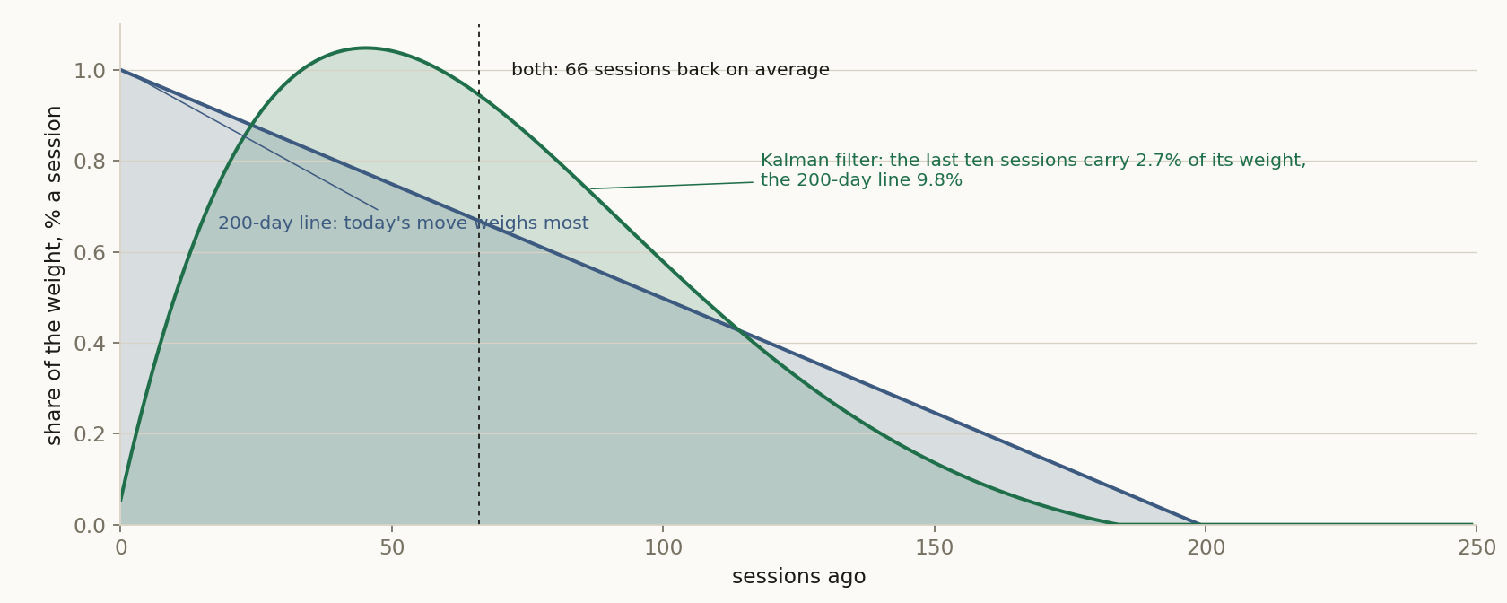
The same horizon. Any trend rule is a weighted average of past price moves (Levine and Pedersen, 2016), and the 200-day line's weights sit on average 66 sessions back. We set the filter's noise so that its weights sit 66 sessions back too, before the test and without looking at a single return. Both rules then run through the same forward test, with the same fills, the whole fund when in and the same cost, so the method is the only difference left between the two.

Different listening. The line gives the most weight to today's move. The filter gives the last ten sessions very little and weighs the moves of about two months ago most. On the way it keeps a better fix on where the price is: over 26 years its estimate of the trend sat on average 2.7% from SPY's close, where the 200-day average sat 6.9% away.

**Figure 1.** What each rule listens to. The share of its weight each rule puts on the price move of each past session, from the rule's own arithmetic. Both average 66 sessions back; the 200-day line weighs today most, the Kalman filter the moves of about two months ago.

**Figure 2.** What each rule sees at two turns. SPY's close, the 200-day average and the Kalman filter's estimate of the trend, from the card's own code; the triangles mark the days each rule left and came back.

1 Methodology, in detail (click to open)

1 Methodology

The walk. Each year from the first of January, both rules traded the fund for one year, from its closes. SPY was walked from 2000 to 2025, QQQ from 2002, gold (GLD) from 2007, and the Russell 2000 fund IWM, the long Treasury fund TLT and the nine sector funds from 2006. Prices are daily closes from a licensed commercial data provider, without dividends, for both rules and for holding the fund alike. A signal is read at the close and the position is held from that close. Every buy and every sell pays 0.02%, and cash earns nothing.

The two rules. The 200-day line holds while the close is above its 200-day average; in the lab it is the Signal Module's moving-average card, the close against its 200-day average. The Kalman filter is the Kalman Trend card on the log of the price with level and slope noise 0.0001 and observation noise 300; it holds while its slope is above zero. Both are set once, before the walk, and never refitted. Both run through the same forward-test engine: the same fills at the close, the whole fund when in the market, 0.02% a trade. The record labels the Kalman side's sizing half-Kelly; that setting is capped at the whole fund, and the whole fund is what it held in every year of every walk.

The fitted twin. The same card was also walked with its horizon and its entry threshold picked before every year by the card's walk-forward, from a ten by ten grid tried on the history before that year. It is the answer to "what if we had fitted it".

The falls. A fall is a decline of 15% or more from a record close on SPY. There were six, and for each we counted when each rule left and how often it bought back in before the bottom.

The record. Every walk is reported: the two versions of the filter against the 200-day line on fourteen funds, 28 walks in all.

2 Results

2.1 Headline

Kalman filter, Sharpe

0.53

day by day, every year the test ran, 2000 to 2025

200-day line, Sharpe

0.42

day by day, every year the test ran, 2000 to 2025

The result

On SPY from 2000 to 2025 the Kalman filter grew 5.8% a year, against 4.1% for the 200-day line and 5.7% for holding the fund, and it left the market 18 times to the line's 92.

show or hide a line: Kalman filter 200-day line platform reference (SPY)

Figure 3. Both arms stitched through the identical windows, Kalman filter (+336.0%), 200-day line (+187.1%), platform reference grey (+322.4%). Dotted verticals mark the step boundaries; the dashed horizontal is break-even. These figures compound each arm's own stitched daily series, the arithmetic of the table below; the paired statistics of 2.4 inner-join both arms' trading days inside each window and start each window after its opening trade, so the two bases differ by that opening charge where the walk pays one. Both are printed from the frozen record.

**Table 1.** Every book in this study on one ruler
Book	Total return	Per year	Volatility	Sharpe	Worst drawdown	Mean window
Kalman filter	+336.0%	5.83%	12.2%	0.53	-29.1%	+6.48%
Benchmark (reference)	+322.4%	5.70%	19.4%	0.38	-58.0%	+7.20%
200-day line	+187.1%	4.14%	11.2%	0.42	-25.7%	+4.95%

Volatility, Sharpe and worst drawdown are computed on each book's own stitched daily series over the identical trading days that Figure 3 draws, so the panel and the figure are the same arithmetic. Sharpe carries no cash hurdle. Mean window is the arithmetic average of the one-year window returns, each from its first close after the opening trade, and does not compound to the total beside it: the difference is volatility drag, plus that opening charge where the walk pays one.

**Figure 4.** Out at the turns. SPY with its six falls of 15% or more from a record close shaded, and below it the days each rule was out of the market.

**Figure 5.** Year by year. The Kalman filter's return minus the 200-day line's, in points; a triangle marks a year inside one of the six falls.

**Figure 6.** Fourteen funds. Growth a year of the 200-day line, the Kalman filter set once and fitted yearly, and holding the fund, prices without dividends; the funds are ordered by how often the line left the market, most at the top.

**Figure 7.** What the walk-forward saw on SPY. The fitted twin's ten by ten grid of in-sample Sharpe ratios, averaged over the 26 years, over the filter's horizon and its entry threshold: a broad plateau at low thresholds from about 58 sessions on.

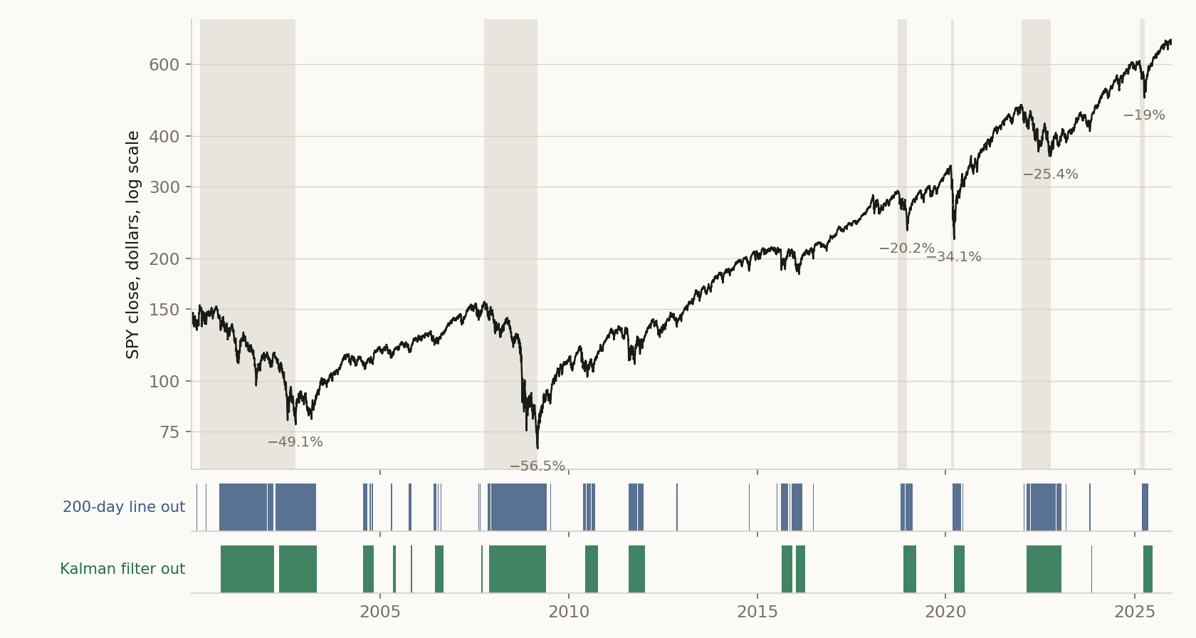
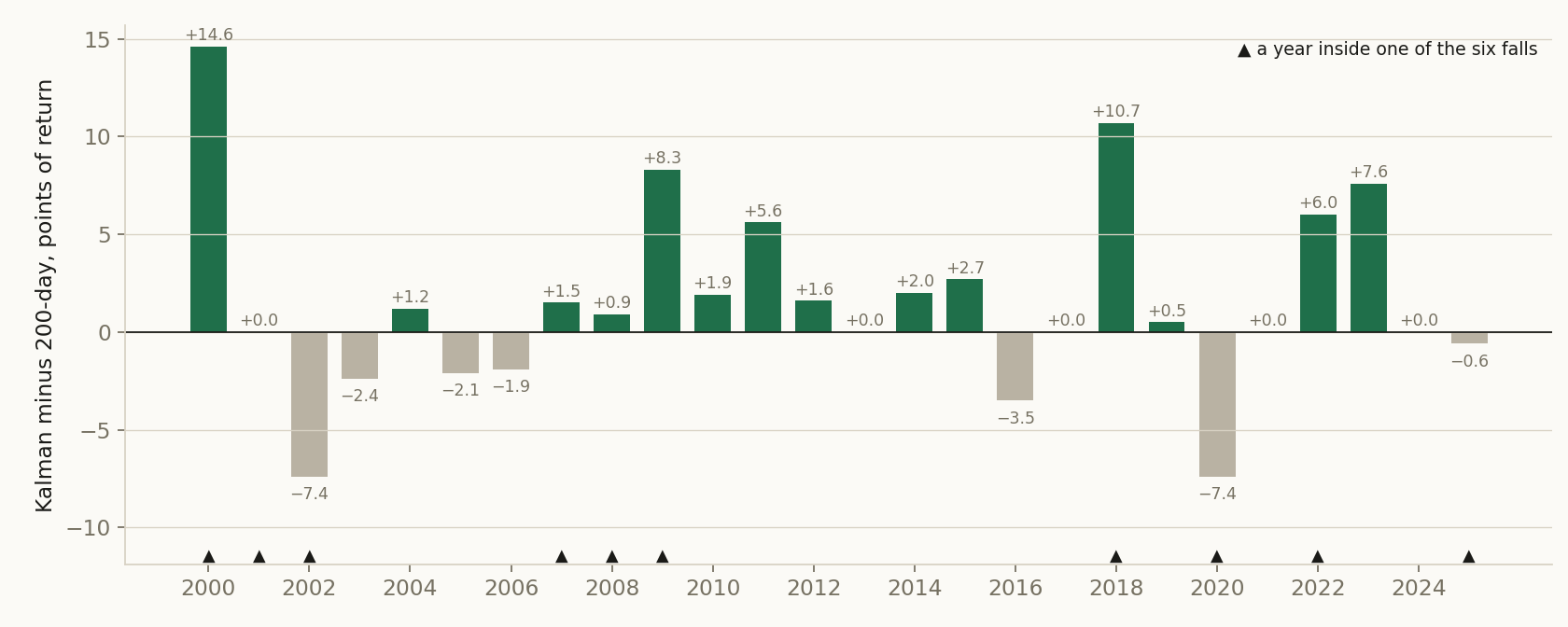
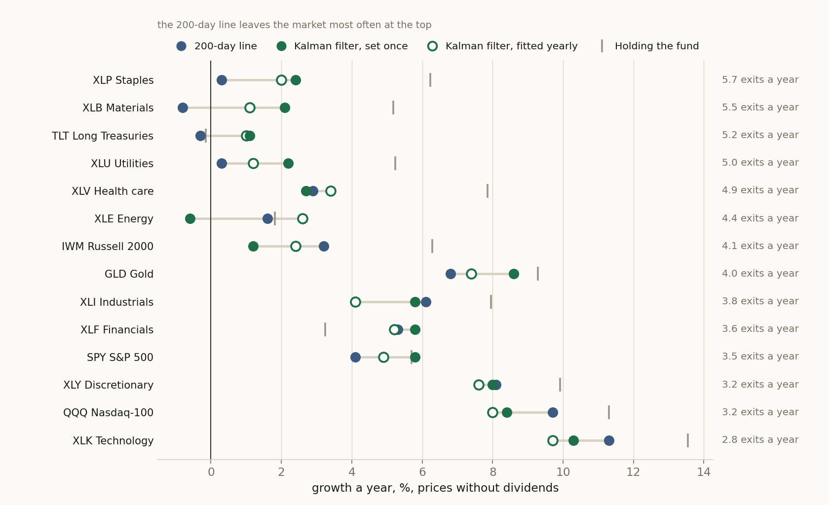
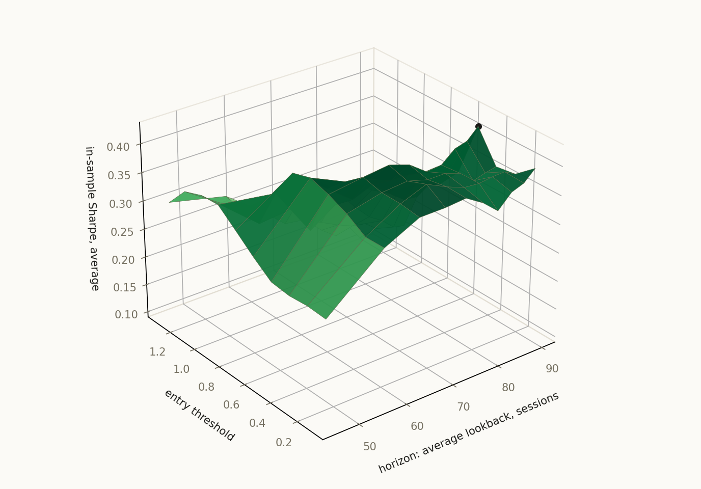
Table 2. The whole record on SPY, 2000 to 2025. Twenty-six one-year windows chained, prices without dividends, 0.02% a trade, cash earns nothing. Sharpe ratio on each book's own daily returns. Bought back higher: exits the rule paid to take.

Book	$10,000 became	A year	Worst drop	Sharpe	Exits	Bought back higher	Invested
Holding SPY	$42,200	5.7%	−58.0%	0.38	-	-	100%
200-day line	$28,700	4.1%	−25.7%	0.42	92	66	72%
Kalman filter, set once	$43,600	5.8%	−29.1%	0.53	18	14	71%
Kalman filter, fitted yearly	$35,100	4.9%	−29.1%	0.46	16	12	68%

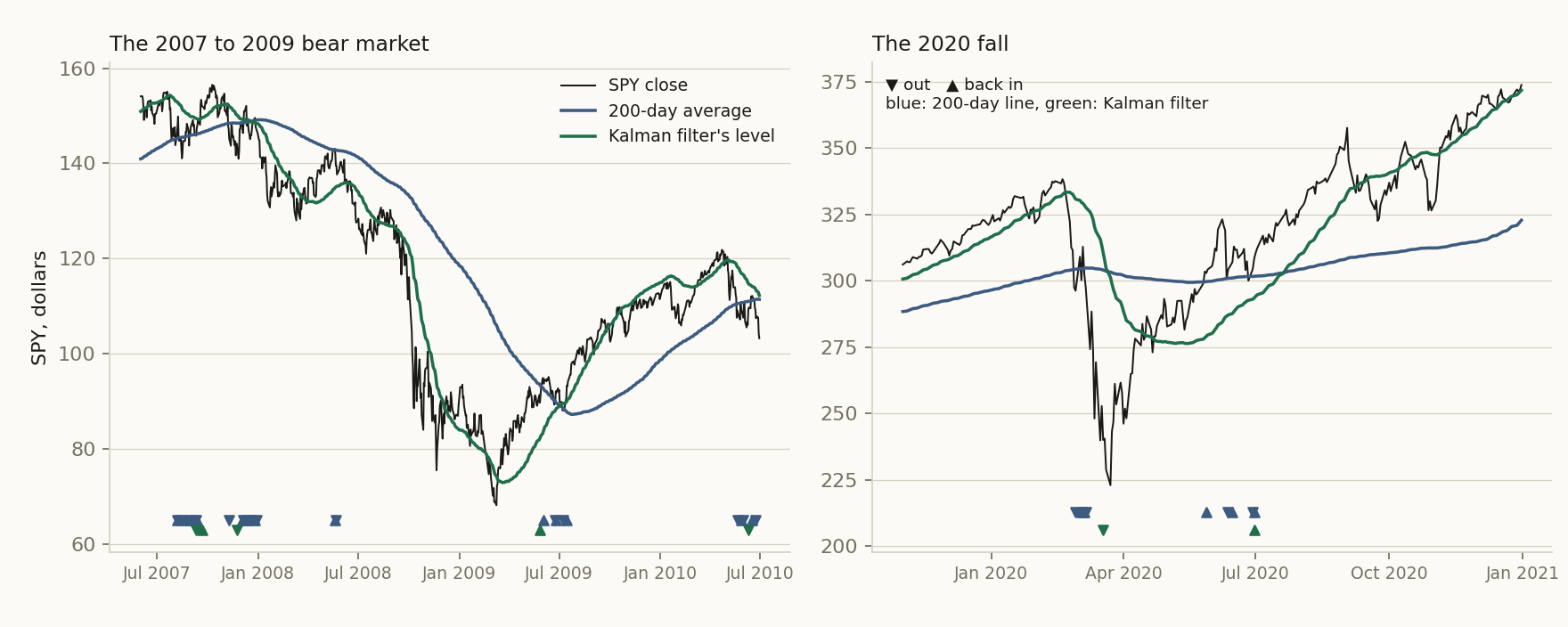
Table 3. SPY's six falls of 15% or more from a record close: when each rule left, and its false starts. Sessions from the record close to the first exit, with the fall already taken. False starts: buys made after the first exit and before the low. The Kalman filter is set once.

Fall	Depth	Left: 200-day line	Left: Kalman filter	False starts: 200-day line	False starts: Kalman filter
Mar 2000 to Oct 2002	−49.1%	16 sessions, at −8.3%	140 sessions, at −13.3%	12	2
Oct 2007 to Mar 2009	−56.5%	22 sessions, at −6.0%	32 sessions, at −7.9%	5	0
Sep 2018 to Dec 2018	−20.2%	16 sessions, at −6.0%	40 sessions, at −7.0%	3	0
Feb 2020 to Mar 2020	−34.1%	7 sessions, at −12.4%	20 sessions, at −29.1%	2	0
Jan 2022 to Oct 2022	−25.4%	14 sessions, at −7.9%	35 sessions, at −11.7%	5	0
Feb 2025 to Apr 2025	−19.0%	14 sessions, at −9.3%	26 sessions, at −7.5%	1	0

Table 4. Fourteen funds: the Kalman filter set once against the 200-day line. Each cell reads Kalman filter / 200-day line. Growth a year and worst drop on prices without dividends, 0.02% a trade; Sharpe ratio on each book's own daily returns; exits from the market a year. SPY from 2000, QQQ from 2002, GLD from 2007, the rest from 2006.

Fund	Growth a year	Holding the fund	Sharpe ratio	Worst drop	Exits a year
SPY S&P 500	5.8% 4.1%	5.7%	0.53 0.42	−29.1% −25.7%	0.7 3.5
QQQ Nasdaq-100	8.4% 9.7%	11.3%	0.58 0.69	−33.4% −25.9%	0.9 3.2
IWM Russell 2000	1.2% 3.2%	6.3%	0.16 0.29	−41.9% −34.2%	1.2 4.1
TLT Long Treasuries	1.1% −0.3%	−0.1%	0.15 0.03	−23.6% −36.7%	1.1 5.2
GLD Gold	8.6% 6.8%	9.3%	0.67 0.55	−35.1% −34.6%	0.8 4.0
XLB Materials	2.1% −0.8%	5.2%	0.21 0.02	−36.6% −46.7%	0.9 5.5
XLE Energy	−0.6% 1.6%	1.8%	0.06 0.18	−50.8% −45.5%	1.0 4.4
XLF Financials	5.8% 5.3%	3.2%	0.45 0.45	−36.7% −26.5%	0.6 3.6
XLI Industrials	5.8% 6.1%	8.0%	0.49 0.52	−32.1% −20.5%	0.8 3.8
XLK Technology	10.3% 11.3%	13.5%	0.68 0.77	−31.5% −25.6%	0.7 2.8
XLP Staples	2.4% 0.3%	6.2%	0.28 0.08	−24.2% −31.1%	0.9 5.7
XLU Utilities	2.2% 0.3%	5.2%	0.23 0.09	−35.7% −33.7%	1.0 5.0
XLV Health care	2.7% 2.9%	7.9%	0.28 0.32	−33.0% −31.8%	0.9 4.9
XLY Discretionary	8.0% 8.1%	9.9%	0.60 0.64	−31.2% −25.4%	0.7 3.2

Sections 2.2 to 3, the full record: every year, every test, and how each one was run (click to open)

The registration names the two groups compared Kalman switch and 200-day switch; this paper calls them Kalman filter and 200-day line.

2.2 Per-step results

**Table 5.** One row per step, raw out-of-sample results. A short window can pair a negative return with a positive annualised Sharpe: at high daily volatility the arithmetic mean of daily returns sits above the compounded window return, and the Sharpe reads the former. Volatility drag, printed rather than smoothed.
#	Out-of-sample window	Kalman filter SR	200-day line SR
1	2000-01-03 → 2000-12-29	-0.21	-1.18
2	2001-01-02 → 2001-12-31	n/a	n/a
3	2002-01-02 → 2002-12-31	-1.94	-1.55
4	2003-01-02 → 2003-12-31	1.81	1.89
5	2004-01-02 → 2004-12-31	0.34	0.21
6	2005-01-03 → 2005-12-30	-0.29	-0.09
7	2006-01-03 → 2006-12-29	0.64	0.88
8	2007-01-03 → 2007-12-31	-0.22	-0.34
9	2008-01-02 → 2008-12-31	n/a	-1.03
10	2009-01-02 → 2009-12-31	1.55	1.08
11	2010-01-04 → 2010-12-31	0.13	-0.01
12	2011-01-03 → 2011-12-30	-0.43	-0.96
13	2012-01-03 → 2012-12-31	0.93	0.83
14	2013-01-02 → 2013-12-31	2.22	2.22
15	2014-01-02 → 2014-12-31	1.10	0.96
16	2015-01-02 → 2015-12-31	-0.54	-0.88
17	2016-01-04 → 2016-12-30	0.53	0.89
18	2017-01-03 → 2017-12-29	2.58	2.58
19	2018-01-02 → 2018-12-31	0.11	-0.76
20	2019-01-02 → 2019-12-31	1.25	1.21
21	2020-01-02 → 2020-12-31	-0.04	0.26
22	2021-01-04 → 2021-12-31	2.02	2.02
23	2022-01-03 → 2022-12-30	-1.43	-2.46
24	2023-01-03 → 2023-12-29	1.34	0.82
25	2024-01-02 → 2024-12-31	1.78	1.78
26	2025-01-02 → 2025-12-31	0.97	1.00

Figure 8. Kalman filter: every step's out-of-sample curve overlaid, each rebased to 1× at its own start. Read alongside the per-step table: consistent shape across steps is the walk-forward's evidence; a single lucky leg is not.

Figure 9. 200-day line: the same windows, the other arm. Compare shape-for-shape with the previous figure: the two arms trade the identical out-of-sample windows.

2.2b Every test, in numbers

Every test this paper registered, two rows each, the paper’s own test first.

Walk	Windows	Span	Growth	CAGR	Worst drawdown	Pooled Sharpe
SPY · Kalman filter, set once (this paper, the one the platform opens)	26	2000-01-03 → 2025-12-31	+336.0%	+5.8%	-29.1%	0.53
SPY · 200-day line (this paper, the one the platform opens)	26	2000-01-03 → 2025-12-31	+187.1%	+4.1%	-25.7%	0.42
SPY · Kalman filter, fitted yearly	26	2000-01-03 → 2025-12-31	+250.6%	+4.9%	-29.1%	0.46
SPY · 200-day line, in the fitted walk	26	2000-01-03 → 2025-12-31	+187.1%	+4.1%	-25.7%	0.42
XLK · Kalman filter, fitted yearly	20	2006-01-03 → 2025-12-31	+540.6%	+9.7%	-31.6%	0.66
XLK · 200-day line, in the fitted walk	20	2006-01-03 → 2025-12-31	+745.2%	+11.3%	-25.6%	0.77
QQQ · Kalman filter, fitted yearly	24	2002-01-02 → 2025-12-31	+534.3%	+8.0%	-28.6%	0.56
QQQ · 200-day line, in the fitted walk	24	2002-01-02 → 2025-12-31	+822.6%	+9.7%	-25.9%	0.69
XLP · Kalman filter, fitted yearly	20	2006-01-03 → 2025-12-31	+48.0%	+2.0%	-26.6%	0.24
XLP · 200-day line, in the fitted walk	20	2006-01-03 → 2025-12-31	+6.3%	+0.3%	-31.1%	0.08
XLB · Kalman filter, fitted yearly	20	2006-01-03 → 2025-12-31	+24.4%	+1.1%	-31.6%	0.15
XLB · 200-day line, in the fitted walk	20	2006-01-03 → 2025-12-31	-14.4%	-0.8%	-46.7%	0.02
IWM · Kalman filter, fitted yearly	20	2006-01-03 → 2025-12-31	+61.5%	+2.4%	-34.1%	0.23
IWM · 200-day line, in the fitted walk	20	2006-01-03 → 2025-12-31	+88.5%	+3.2%	-34.2%	0.29
XLU · Kalman filter, fitted yearly	20	2006-01-03 → 2025-12-31	+28.0%	+1.2%	-36.5%	0.16
XLU · 200-day line, in the fitted walk	20	2006-01-03 → 2025-12-31	+6.6%	+0.3%	-33.7%	0.09
XLE · Kalman filter, fitted yearly	20	2006-01-03 → 2025-12-31	+66.3%	+2.6%	-37.3%	0.23
XLE · 200-day line, in the fitted walk	20	2006-01-03 → 2025-12-31	+37.2%	+1.6%	-45.5%	0.18
TLT · Kalman filter, fitted yearly	20	2006-01-03 → 2025-12-31	+21.4%	+1.0%	-29.9%	0.15
TLT · 200-day line, in the fitted walk	20	2006-01-03 → 2025-12-31	-5.8%	-0.3%	-36.7%	0.03
XLV · Kalman filter, fitted yearly	20	2006-01-03 → 2025-12-31	+96.6%	+3.4%	-38.0%	0.34
XLV · 200-day line, in the fitted walk	20	2006-01-03 → 2025-12-31	+78.0%	+2.9%	-31.8%	0.32
XLF · Kalman filter, fitted yearly	20	2006-01-03 → 2025-12-31	+175.9%	+5.2%	-35.9%	0.42
XLF · 200-day line, in the fitted walk	20	2006-01-03 → 2025-12-31	+182.2%	+5.3%	-26.5%	0.45
GLD · Kalman filter, fitted yearly	19	2007-01-03 → 2025-12-31	+289.4%	+7.4%	-35.2%	0.60
GLD · 200-day line, in the fitted walk	19	2007-01-03 → 2025-12-31	+251.0%	+6.8%	-34.6%	0.55
XLI · Kalman filter, fitted yearly	20	2006-01-03 → 2025-12-31	+123.8%	+4.1%	-39.8%	0.36
XLI · 200-day line, in the fitted walk	20	2006-01-03 → 2025-12-31	+224.9%	+6.1%	-20.5%	0.52
XLY · Kalman filter, fitted yearly	20	2006-01-03 → 2025-12-31	+335.7%	+7.6%	-28.9%	0.59
XLY · 200-day line, in the fitted walk	20	2006-01-03 → 2025-12-31	+375.3%	+8.1%	-25.4%	0.64
XLB · Kalman filter, set once	20	2006-01-03 → 2025-12-31	+50.7%	+2.1%	-36.6%	0.21
XLB · 200-day line	20	2006-01-03 → 2025-12-31	-14.4%	-0.8%	-46.7%	0.02
XLE · Kalman filter, set once	20	2006-01-03 → 2025-12-31	-11.8%	-0.6%	-50.8%	0.06
XLE · 200-day line	20	2006-01-03 → 2025-12-31	+37.2%	+1.6%	-45.5%	0.18
QQQ · Kalman filter, set once	24	2002-01-02 → 2025-12-31	+599.0%	+8.4%	-33.4%	0.58
QQQ · 200-day line	24	2002-01-02 → 2025-12-31	+822.6%	+9.7%	-25.9%	0.69
XLP · Kalman filter, set once	20	2006-01-03 → 2025-12-31	+61.1%	+2.4%	-24.2%	0.28
XLP · 200-day line	20	2006-01-03 → 2025-12-31	+6.3%	+0.3%	-31.1%	0.08
XLF · Kalman filter, set once	20	2006-01-03 → 2025-12-31	+209.8%	+5.8%	-36.7%	0.45
XLF · 200-day line	20	2006-01-03 → 2025-12-31	+182.2%	+5.3%	-26.5%	0.45
XLU · Kalman filter, set once	20	2006-01-03 → 2025-12-31	+54.1%	+2.2%	-35.7%	0.23
XLU · 200-day line	20	2006-01-03 → 2025-12-31	+6.6%	+0.3%	-33.7%	0.09
IWM · Kalman filter, set once	20	2006-01-03 → 2025-12-31	+28.0%	+1.2%	-41.9%	0.16
IWM · 200-day line	20	2006-01-03 → 2025-12-31	+88.5%	+3.2%	-34.2%	0.29
XLI · Kalman filter, set once	20	2006-01-03 → 2025-12-31	+210.0%	+5.8%	-32.1%	0.49
XLI · 200-day line	20	2006-01-03 → 2025-12-31	+224.9%	+6.1%	-20.5%	0.52
XLV · Kalman filter, set once	20	2006-01-03 → 2025-12-31	+69.2%	+2.7%	-33.0%	0.28
XLV · 200-day line	20	2006-01-03 → 2025-12-31	+78.0%	+2.9%	-31.8%	0.32
TLT · Kalman filter, set once	20	2006-01-03 → 2025-12-31	+23.9%	+1.1%	-23.6%	0.15
TLT · 200-day line	20	2006-01-03 → 2025-12-31	-5.8%	-0.3%	-36.7%	0.03
XLK · Kalman filter, set once	20	2006-01-03 → 2025-12-31	+612.0%	+10.3%	-31.5%	0.68
XLK · 200-day line	20	2006-01-03 → 2025-12-31	+745.2%	+11.3%	-25.6%	0.77
XLY · Kalman filter, set once	20	2006-01-03 → 2025-12-31	+361.6%	+8.0%	-31.2%	0.60
XLY · 200-day line	20	2006-01-03 → 2025-12-31	+375.3%	+8.1%	-25.4%	0.64
GLD · Kalman filter, set once	19	2007-01-03 → 2025-12-31	+379.6%	+8.6%	-35.1%	0.67
GLD · 200-day line	19	2007-01-03 → 2025-12-31	+251.0%	+6.8%	-34.6%	0.55
platform reference (SPY) (benchmark)		2000-01-03 → 2025-12-31	+322.4%	+5.7%	-58.0%

Growth and CAGR above are each walk over its own windows, so they are not comparable across walks with different window counts: a walk that excluded a window did not live through it. The figure rebases every line on the session all of them share.

2.3 Search accounting

This paper's search is a declared family: the paper's 28 walks, counted at N = 28 evaluated books. Every member is either a registered walk with its own hypothesis and frozen record, or a derived average computed from those frozen records; every member is reported, in the family table, and none was selected away. The count is declared by the author rather than derived from one project's ledger, because the members are sibling registered studies; the declaration names them and is frozen in this artifact. What the source strategy's author searched before publishing is not knowable from here and is not counted. The registered per-step record below still guarantees each window's hypothesis was hashed and registered before that window was scored.

2.4 The comparison

Both arms trade the same registered windows, so their returns can be PAIRED: inside each window the two return series are inner-joined date by date and the difference r_{Kalman filter} − r_{200-day line} is the object under test. Because this is ONE pre-declared contrast, frozen at registration before any window was scored, the paired statistic needs no multiple-testing deflation; the arm-level records carry the declared family count of §2.3 as their search accounting, and this contrast, registered per window before scoring, is not multiplied by it.

**Table 6.** Window-by-window paired comparison. Δ is the growth gap (Kalman filter − 200-day line) over the window's paired dates.
#	Window	Paired bars	Kalman filter	200-day line	Δ	Leader
1	2000-01-04 → 2000-12-29	251	-6.1%	-20.8%	+14.6 pp	Kalman filter
2	2001-01-03 → 2001-12-31	247	+0.0%	+0.0%	+0.0 pp	tie
3	2002-01-03 → 2002-12-31	251	-11.8%	-4.4%	-7.4 pp	200-day line
4	2003-01-03 → 2003-12-31	251	+20.8%	+23.2%	-2.4 pp	200-day line
5	2004-01-05 → 2004-12-31	251	+2.7%	+1.6%	+1.2 pp	Kalman filter
6	2005-01-04 → 2005-12-30	251	-3.2%	-1.2%	-2.0 pp	200-day line
7	2006-01-04 → 2006-12-29	250	+5.3%	+7.2%	-1.9 pp	200-day line
8	2007-01-04 → 2007-12-31	250	-3.9%	-5.4%	+1.4 pp	Kalman filter
9	2008-01-03 → 2008-12-31	252	+0.0%	-0.9%	+0.9 pp	Kalman filter
10	2009-01-05 → 2009-12-31	251	+22.0%	+13.7%	+8.3 pp	Kalman filter
11	2010-01-05 → 2010-12-31	251	+0.8%	-1.0%	+1.9 pp	Kalman filter
12	2011-01-04 → 2011-12-30	251	-5.4%	-11.0%	+5.6 pp	Kalman filter
13	2012-01-04 → 2012-12-31	249	+11.5%	+9.9%	+1.6 pp	Kalman filter
14	2013-01-03 → 2013-12-31	251	+26.4%	+26.4%	+0.0 pp	tie
15	2014-01-03 → 2014-12-31	251	+12.4%	+10.3%	+2.1 pp	Kalman filter
16	2015-01-05 → 2015-12-31	251	-6.4%	-9.1%	+2.7 pp	Kalman filter
17	2016-01-05 → 2016-12-30	251	+4.7%	+8.2%	-3.5 pp	200-day line
18	2017-01-04 → 2017-12-29	250	+18.5%	+18.5%	+0.0 pp	tie
19	2018-01-03 → 2018-12-31	250	+0.5%	-10.2%	+10.7 pp	Kalman filter
20	2019-01-03 → 2019-12-31	251	+14.0%	+13.5%	+0.5 pp	Kalman filter
21	2020-01-03 → 2020-12-31	252	-4.5%	+3.0%	-7.4 pp	200-day line
22	2021-01-05 → 2021-12-31	251	+28.8%	+28.8%	+0.0 pp	tie
23	2022-01-04 → 2022-12-30	250	-10.1%	-16.1%	+6.0 pp	Kalman filter
24	2023-01-04 → 2023-12-29	249	+17.0%	+9.4%	+7.6 pp	Kalman filter
25	2024-01-03 → 2024-12-31	251	+24.0%	+24.0%	+0.0 pp	tie
26	2025-01-03 → 2025-12-31	249	+10.5%	+11.0%	-0.5 pp	200-day line

Paired Sharpe of the difference track: 0.26 · block bootstrap (2000 paths, block 10, seed 1234): P(Kalman filter beats 200-day line) = 95.4%.

Window win-rate. Kalman filter led 14 of 26 windows (53.8%), 200-day line led 7, and 5 windows were ties, and the mean window gap of +1.53 pp points the same way. Widest single window: 2000 at +14.6 pp.

3 The circuit

The strategy is a circuit of platform primitives, frozen when the study is registered. Below is the circuit as wired on the canvas, the objective it encodes and how the search runs through it, followed by the mathematics each primitive actually computes, the same formulas the execution engine runs. The complete parameterisation is preserved in the study ledger (Appendix A).

The hypothesis under test

The sentence below is the registered design with its rules in plain words; the exact registration record is in Appendix A2; the authored description of the design is Section 1.

A COMPARATIVE study: Kalman switch vs 200-day switch, walked on the same registered out-of-sample windows. Kalman switch: SPY, traded via Kalman Trend Filter signal, and forward-tested out-of-sample from the anchor: the rule set is frozen at the anchor, with no in-sample re-optimization. 200-day switch: SPY, bought when the close is above its 200-day average; sell when the close is below its 200-day average, and forward-tested out-of-sample from the anchor: the rule set is frozen at the anchor, with no in-sample re-optimization. The arms differ in: 2 places: Kalman Trend Filter → Signal Module, substituted (its parameters change with the swap); Stoch Forward Test → Signal Forward Test, substituted (its parameters change with the swap). NOTE: with more than one difference, an out-of-sample gap cannot be attributed to any single change. The contrast under test: whether Kalman switch generates better risk-adjusted returns than 200-day switch over the identical out-of-sample windows.

Every block in this study is a card from the platform's catalog: the ticker and its price loader, the Kalman Trend card on the log of the price, the forward test, the Signal Module with the 200-day rule and the cost card. The card's log-of-the-price option shipped before these walks ran, so a reader can rebuild every walk.

Figure 10. The frozen circuit, every node a primitive, every wire a typed data-flow; the two arms are colour-coded (Kalman filter green, 200-day line blue, shared feeds neutral). Each box is one step of the strategy; data flows along the wires left to right, and no box can see data dated later than the box feeding it. The whole diagram was frozen when the hypothesis was registered. Click any node to open what that step ran with and what it produced.

Envelopes show counts, ratios, dates, and the parameters the author chose. Full price and per-name data series are not republished: the underlying market data is licensed to QuanterLab. Point figures quoted in the prose, a named holding's return over a stated span, are summary facts derived from public market prices, not redistributed series.

What each part does

Ticker, A single instrument symbol, the seed of a single-name circuit.

Ticker Price Loader, Single-ticker OHLCV loader, the deep window a signal needs.

Stoch Kalman Trend, Kalman trend, track level AND slope; trade the slope.

Signal Module, The entry / exit rule, turn indicators into a per-bar trade signal.

Stochastic Forward, Forward-test an OU / Kalman rule on unseen data.

Transaction Cost, Charge for trading, slippage + commission on every turn.

Backtest Validator, Forward-test the winning rule on unseen, out-of-sample data.

The objective and the search

Kalman switch

Universe	Single ticker SPY with 365 days (~1.0y) of price history.
Signal generation	Kalman Trend Filter signal.
Validation & out-of-sample	stochastic forward test (1y horizon from the anchor); overlays: Transaction Cost.

200-day switch

Signal generation	buy when the close is above its 200-day average; sell when the close is below its 200-day average.
Validation & out-of-sample	signal forward test (1y horizon from the anchor); overlays: Transaction Cost.

Every other specification row is identical to Kalman switch's table above.

What differs between the arms, 2 differences; more than one thing changes at once:

substitutedKalman Trend Filter → Signal Module, substituted (its parameters change with the swap)
substitutedStoch Forward Test → Signal Forward Test, substituted (its parameters change with the swap)

Reader's note. With 2 settings changed at once across 2 nodes, an out-of-sample gap between the arms cannot be attributed to any single change, the arms are compared as whole packages, and any causal reading of one ingredient is unsupported by this design.

Cost elements are wired into the circuit.

Show the mathematics, 7 primitives, formulas and parity notes

3.1 Ticker

A single instrument symbol, the seed of a single-name circuit.

No math. It just names one stock and hands the symbol to a Ticker Price Loader, which fetches its price history.

What it is

A constant: one ticker string. The computation lives downstream in the loader and the signal.

3.2 Ticker Price Loader

Single-ticker OHLCV loader, the deep window a signal needs.

Same as the bulk loader but for one name, fetching a deep lifecycle window so an indicator or stochastic signal has enough history to warm up.

What it loads

One ticker's OHLCV up to the anchor, length set by the strategy's warm-up requirement.

P = \{(o,h,l,c,v)_\tau : \tau \le t\}

3.3 Stoch Kalman Trend

Kalman trend, track level AND slope; trade the slope.

A 2-D local-linear-trend Kalman filter carries both a level and a slope as hidden state. The signal is the slope expressed in standard deviations, positive and significant means an established uptrend; crossing zero flags the turn.

Local linear trend state

\begin{bmatrix} \ell_t \\ s_t \end{bmatrix} = \begin{bmatrix} 1 & 1 \\ 0 & 1 \end{bmatrix}\begin{bmatrix} \ell_{t-1} \\ s_{t-1} \end{bmatrix} + \eta_t

ℓ = level, s = slope; Q_level and Q_trend set how fast each adapts (Joseph-form covariance).

Trend z-score

z_t = \frac{s_t}{\sqrt{P_t[1,1]}}\ \ (\text{clipped }\pm 5)

Enter when z > trend_threshold; exit when z < trend_exit_z (0 = zero-cross).

Byte-identical to SC001STCB (shared_libs/stochastic_core).

3.4 Stochastic Forward

Forward-test an OU / Kalman rule on unseen data.

Takes the validated stochastic configuration and trades it bar-by-bar on a forward window it has never seen, producing the out-of-sample equity curve, trades and statistics.

Apply the rule forward

\text{enter at } \lvert z_t\rvert > z_{\text{entry}},\ \ \text{exit at } \lvert z_t\rvert < z_{\text{exit}}

Position sizing applied per the sizing panel; returns the terminal result.

3.5 Transaction Cost

Charge for trading, slippage + commission on every turn.

Real trading isn't free. This deducts a cost proportional to how much you trade (turnover), in basis points, so the backtest reflects net, not gross, performance.

Cost per rebalance

\text{cost}_t = \frac{\text{bps}}{10{,}000}\;\times\;\text{turnover}_t, \qquad \text{turnover}_t = \tfrac12\sum_i \lvert w_{i,t}-w_{i,t^-}\rvert

3.6 Signal Module

The entry / exit rule, turn indicators into a per-bar trade signal.

Composes indicators (RSI, moving averages, …) with comparison and logic operators into a rule that says enter, exit, or hold each bar. The rule is emitted as a portable config the optimizer tunes and the walk-forward validates, so what you design is exactly what gets traded.

Boolean rule → position state

\text{signal}_t = \begin{cases} +1 & \text{entry rule true} \\ 0 & \text{exit rule true} \\ \text{hold} & \text{otherwise}\end{cases}

e.g. enter when RSI < 30, exit when RSI > 50.

3.7 Backtest Validator

Forward-test the winning rule on unseen, out-of-sample data.

Takes the wired rule config (the Walk-Forward validated config wins, else the optimized config, else the raw signal config) and trades it FORWARD on the out-of-sample window to the right of the anchor, data it never saw during optimization, re-deriving the regime as-of each bar. It produces the true out-of-sample equity curve, trades and statistics: the signal-path twin of the Portfolio Forward Test, not an in-sample replay.

Apply the frozen rule forward (OOS)

E_t = E_{t-1}\,(1 + r_t),\qquad \text{Sharpe} = \frac{\bar r - r_f}{\sigma_r}\sqrt{252}

Config frozen from optimization / walk-forward, then replayed bar-by-bar on the forward window it has never seen, with cost + risk overlays applied.

4 Discussion

4.1 Findings

The whole record. Over the 26 years SPY grew 5.8% a year with the filter, 4.1% with the 200-day line and 5.7% held, and the filter's worst drop was half the fund's. It was ahead of the line in 14 of the 26 years.

Where the gap came from. Two thirds of it came from the ten years that held one of SPY's six falls of 15% or more from a record close. Inside those falls the line bought back in 28 times before the bottom, 12 of them in the 2000 to 2002 bear market, where the price crossed its average again and again on the way down; the filter did so twice. The line left first in every fall, and the filter paid for its lag in the fast fall of 2020.

Thirteen more funds. The filter left the market less than a third as often as the line on every fund, about a fifth as often on average. It grew more on seven of the fourteen, with an equal or better Sharpe ratio on the same seven, and it tended to gain most where the line went in and out most often. Its worst drop was deeper than the line's on eleven of them.

Fitting it every year. The fitted twin grew more than the line on eight of the fourteen funds, and on SPY it landed between the two (4.9% a year). Its grid is a broad plateau rather than a sharp peak, and the horizon we fixed before the walk lies inside it.

4.2 Interpretation

Why the model ended ahead. The line reacts to today's price, so it is quick at the top, and quick to be fooled when a falling market bounces or a calm one wobbles. The filter barely hears the last few days, so it is late at every turn and rarely fooled. On SPY the false alarms it skipped were worth more than the weeks it lost.

Where the story stops. The filter did not beat the line on every fund, and before dividends it beat holding the fund on three of the fourteen. What it does on every one is leave the market far less often. The fitted twin's plateau reaches the edge of our grid, so longer horizons, for both methods, are the next test. The record of all 28 walks is below, and the circuit opens in the lab.

Enter the lab

Press Open the platform and this paper's circuit opens in the lab: the fund and its prices, the Kalman Trend card on the log of the price with observation noise 300, the forward test, and beside it the 200-day line, the Signal Module's moving-average card.

Things to try. Raise the observation noise to 1000 or 3000 and see whether the plateau goes on past the edge of our grid. Change the fund to gold or long Treasuries. Put the noise in price units and watch the filter react to every move. Or give the 200-day rule a longer or shorter average and see how the gap between the two methods moves.

4.3 Limitations

Prices leave out dividends, for both rules and for holding the fund, and cash earns nothing; with dividends and a Treasury-bill rate every book would grow more, and the two rules, invested about seven days in ten, would gain less from dividends and more from the bills than holding. There is one trading cost, 0.02% a trade. The filter's horizon was matched to the line's by a rule fixed before the walk; the fitted twin shows one way the choice could have gone. Two earlier designs of this comparison, 36 walks registered and scored the same morning with the filter set up differently (its noise in dollars, then a one-month horizon), stay on the platform's record and are not counted in the 28 reported here.

References

QuanterLab reference architecture

Gelman, A., & Loken, E. (2013). The garden of forking paths: Why multiple comparisons can be a problem, even when there is no “fishing expedition.” Working paper, Columbia University.
Harvey, C. R., Liu, Y., & Zhu, H. (2016). … and the Cross-Section of Expected Returns. Review of Financial Studies, 29(1), 5–68. doi:10.1093/rfs/hhv059
Lo, A. W. (2002). The Statistics of Sharpe Ratios. Financial Analysts Journal, 58(4), 36–52. doi:10.2469/faj.v58.n4.2453

Author’s references?

Faber (2007), A Quantitative Approach to Tactical Asset Allocation, Journal of Wealth Management 9(4): a ten-month moving average rule kept the returns of US stocks and several other asset classes while cutting their drawdowns. https://doi.org/10.3905/jwm.2007.674809
Brock, Lakonishok and LeBaron (1992), Simple Technical Trading Rules and the Stochastic Properties of Stock Returns, Journal of Finance 47(5): moving-average rules on the Dow from 1897 to 1986 had returns that standard models of prices could not explain. https://doi.org/10.1111/j.1540-6261.1992.tb04681.x
Kalman (1960), A New Approach to Linear Filtering and Prediction Problems, Journal of Basic Engineering 82(1): the filter itself, a recursive estimate of a hidden state from noisy measurements. https://doi.org/10.1115/1.3662552
Harvey (1989), Forecasting, Structural Time Series Models and the Kalman Filter, Cambridge University Press: the local linear trend model, a level and a slope that each wander, which the Kalman Trend card uses. https://doi.org/10.1017/CBO9781107049994
Levine and Pedersen (2016), Which Trend Is Your Friend?, Financial Analysts Journal 72(3): moving averages, time-series momentum and linear filters such as the Kalman filter are all weighted averages of past returns and differ in the horizon they read. https://doi.org/10.2469/faj.v72.n3.3
Bruder, Dao, Richard and Roncalli (2011), Trend Filtering Methods for Momentum Strategies, Lyxor white paper: for a price that is a random walk plus noise, the Kalman filter is the best exponential moving average. https://papers.ssrn.com/sol3/papers.cfm?abstract_id=2289097
Zakamulin (2014), The real-life performance of market timing with moving average and time-series momentum rules, Journal of Asset Management 15(4): after costs and out of sample, moving-average timing on US stocks kept its lower risk but lost much of its return edge. https://doi.org/10.1057/jam.2014.25
Hurst, Ooi and Pedersen (2017), A Century of Evidence on Trend-Following Investing, Journal of Portfolio Management 44(1): trend following earned positive returns in every decade since 1880 and did best in the largest market falls. https://doi.org/10.3905/jpm.2017.44.1.015
Bailey and Lopez de Prado (2014), The Deflated Sharpe Ratio, Journal of Portfolio Management 40(5): how much a Sharpe ratio must be discounted for the number of trials behind it. https://doi.org/10.3905/jpm.2014.40.5.094

Appendix A Reproducibility in QuanterLab

Each step is backed by a frozen run report. The study is re-derivable from the ledger below.

#	Commit	Report	Anchor	OOS window
1	2a24fd87365c	12052	2000-01-01	2000-01-03 → 2000-12-29
2	afc0fb6c7f6d	12053	2001-01-01	2001-01-02 → 2001-12-31
3	c22489845fc2	12054	2002-01-01	2002-01-02 → 2002-12-31
4	1a5a03b22f7f	12055	2003-01-01	2003-01-02 → 2003-12-31
5	88f00b46fa27	12058	2004-01-01	2004-01-02 → 2004-12-31
6	cc6bc5e7cb48	12059	2005-01-01	2005-01-03 → 2005-12-30
7	0ac63781f6b3	12060	2006-01-01	2006-01-03 → 2006-12-29
8	7b015c7161b3	12061	2007-01-01	2007-01-03 → 2007-12-31
9	28cbb9545995	12064	2008-01-01	2008-01-02 → 2008-12-31
10	2b6d76a43305	12065	2009-01-01	2009-01-02 → 2009-12-31
11	560636abaf2c	12066	2010-01-01	2010-01-04 → 2010-12-31
12	d6eda370c83d	12068	2011-01-01	2011-01-03 → 2011-12-30
13	7465250797aa	12070	2012-01-01	2012-01-03 → 2012-12-31
14	5413ed992de8	12071	2013-01-01	2013-01-02 → 2013-12-31
15	57f8ade1499c	12072	2014-01-01	2014-01-02 → 2014-12-31
16	1b4197398d4b	12074	2015-01-01	2015-01-02 → 2015-12-31
17	dab57c84f0c4	12076	2016-01-01	2016-01-04 → 2016-12-30
18	bf829c2eef46	12077	2017-01-01	2017-01-03 → 2017-12-29
19	fae0d1f2e186	12078	2018-01-01	2018-01-02 → 2018-12-31
20	64f5bb23b177	12081	2019-01-01	2019-01-02 → 2019-12-31
21	a67f6a2925ef	12082	2020-01-01	2020-01-02 → 2020-12-31
22	a2294ccf94d9	12083	2021-01-01	2021-01-04 → 2021-12-31
23	46ffce0e1a11	12086	2022-01-01	2022-01-03 → 2022-12-30
24	4e1840ad7aa8	12087	2023-01-01	2023-01-03 → 2023-12-29
25	24c2472cc1a3	12088	2024-01-01	2024-01-02 → 2024-12-31
26	7ada3daf2c7c	12090	2025-01-01	2025-01-02 → 2025-12-31

Appendix A2 Registration record

What this record does and does not establish. Every window in this study is historical: the data existed before the study began, so this is sequential registration on past windows, not pre-registration in the clinical-trial sense, and no procedure could make it so. What the platform does enforce is order, each step's specification was frozen and hashed before that step was scored, and the walk cannot advance past a step that was never run or close one with a result registered for a different window. The two timestamp columns below are the evidence: read them together and each registration precedes its own run, and each run precedes the next registration. A study whose registrations all post-date its runs would show it here. Wall-clock spacing between registrations varies with the author's schedule and queue latency; the ordering, not the tempo, is the claim.

“A COMPARATIVE study: Kalman switch vs 200-day switch, walked on the same registered out-of-sample windows. Kalman switch: SPY, traded via Kalman Trend Filter signal, and forward-tested out-of-sample from the anchor: the rule set is frozen at the anchor, with no in-sample re-optimization. 200-day switch: SPY, bought when the close is above its 200-day average; sell when the close is below its 200-day average, and forward-tested out-of-sample from the anchor: the rule set is frozen at the anchor, with no in-sample re-optimization. The arms differ in: 2 places: Kalman Trend Filter → Signal Module, substituted (its parameters change with the swap); Stoch Forward Test → Signal Forward Test, substituted (its parameters change with the swap). NOTE: with more than one difference, an out-of-sample gap cannot be attributed to any single change. The contrast under test: whether Kalman switch generates better risk-adjusted returns than 200-day switch over the identical out-of-sample windows.”

The same hypothesis was registered independently at every step, hashed before each step's out-of-sample window was scored:

**Table 7.** Registration audit, one row per registered step, with the time each specification was frozen and the time its window was scored. The hypothesis is identical on every row by design: it was registered once and re-registered unchanged at each anchor. Rows that differ would mean the specification moved mid-walk, which is the thing this record exists to rule out. The timestamps are the separate claim: each registration precedes its own run, and each run precedes the next registration.
#	Anchor	Registered at (UTC)	Run completed (UTC)
1	2000-01-01	2026-09-28 08:34:08	2026-09-28 08:34:16
2	2001-01-01	2026-09-28 08:34:16	2026-09-28 08:34:24
3	2002-01-01	2026-09-28 08:34:24	2026-09-28 08:34:33
4	2003-01-01	2026-09-28 08:34:33	2026-09-28 08:34:41
5	2004-01-01	2026-09-28 08:34:41	2026-09-28 08:34:49
6	2005-01-01	2026-09-28 08:34:49	2026-09-28 08:34:58
7	2006-01-01	2026-09-28 08:34:58	2026-09-28 08:35:06
8	2007-01-01	2026-09-28 08:35:06	2026-09-28 08:35:14
9	2008-01-01	2026-09-28 08:35:14	2026-09-28 08:35:23
10	2009-01-01	2026-09-28 08:35:23	2026-09-28 08:35:31
11	2010-01-01	2026-09-28 08:35:32	2026-09-28 08:35:40
12	2011-01-01	2026-09-28 08:35:40	2026-09-28 08:35:48
13	2012-01-01	2026-09-28 08:35:48	2026-09-28 08:35:57
14	2013-01-01	2026-09-28 08:35:57	2026-09-28 08:36:05
15	2014-01-01	2026-09-28 08:36:05	2026-09-28 08:36:14
16	2015-01-01	2026-09-28 08:36:14	2026-09-28 08:36:22
17	2016-01-01	2026-09-28 08:36:22	2026-09-28 08:36:30
18	2017-01-01	2026-09-28 08:36:31	2026-09-28 08:36:39
19	2018-01-01	2026-09-28 08:36:39	2026-09-28 08:36:47
20	2019-01-01	2026-09-28 08:36:47	2026-09-28 08:36:56
21	2020-01-01	2026-09-28 08:36:56	2026-09-28 08:37:04
22	2021-01-01	2026-09-28 08:37:04	2026-09-28 08:37:13
23	2022-01-01	2026-09-28 08:37:13	2026-09-28 08:37:21
24	2023-01-01	2026-09-28 08:37:21	2026-09-28 08:37:29
25	2024-01-01	2026-09-28 08:37:30	2026-09-28 08:37:38
26	2025-01-01	2026-09-28 08:37:38	2026-09-28 08:37:46

Appendix B Per-step diagnostics

Realized in the projection tables below is the risk engine scoring its own forecast: the buy-and-hold return of the segment that followed each rebalance, on the same gross basis the cone was projected on. It is deliberately not the charged, calendar-window total return the study’s tables print, so the two will not reconcile line by line; the cone and its outcome share one basis, which is what a calibration test requires. Each row names its segment’s span so a boundary session is visible.

Names held is the union across the window: the count of distinct instruments the book touched between the window’s first and last session, not the number it held at one time. A book that rotates monthly touches more names than it holds.

What each step's run actually did beyond its return: capital allocation across lanes and regimes, the portfolio book's rebalancing and cost drag, and how positions were sized. Harvested from the frozen run reports, present where the circuit produced them. Cost drag is the gap between the step's return before and after its trading costs, in percentage points of the step's starting capital, so on a book that trades every session and compounds it can exceed the step's own net return.

Open the full per-step grid (26 steps: every rebalance, capital routing and sizing, per window)