

What a European country fund is made of, and whether the country part is worth rotating
Every European rotation system in circulation treats the country as the unit of risk. The people who run these books rank Germany against Spain against Sweden and call the result a country bet. A European country index is a concentrated sector bet: banks carry the south, pharma and staples carry Switzerland. So the question here is whether European country rotation is already sector rotation, and whether the reader should trade the sectors instead.
That industry explains more of a developed-market return than country does has stood since Cavaglia, Brightman and Aked in 2000. Single-country funds have kept selling on the country premise ever since, and nobody had run the question on the ten funds a retail account can hold. Answering it needs a mimic refitted every month and thirty separate walks, which is laborious rather than hard, and laborious is usually enough to stop a thing being done.
I registered one expectation before any window ran. What the sectors cannot explain should matter most under stress, because that is when a country's own banks and its own politics pull it away from the pack.
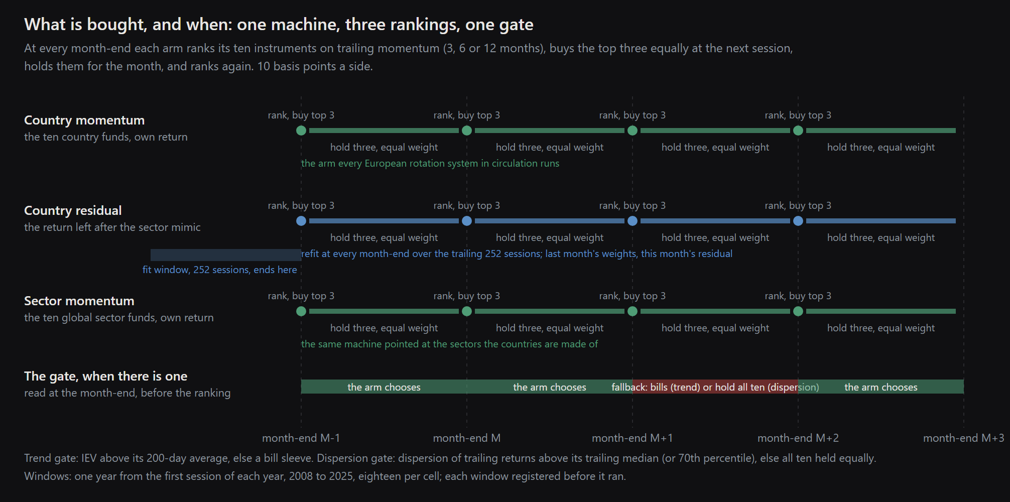
To test it, each of the ten country funds is fitted at every month-end to ten global sector funds as a long-only portfolio, so the weights read as a holding a person could own rather than as a regression. Three arms then rotate monthly on the same machine and differ only in what they rank: the countries on their own return, the countries on the return the fit leaves over, and the sectors themselves. Three lookbacks and three gates make thirty sealed studies, each walked through eighteen one-year windows from 2008, every window registered before it was scored.
Three quarters of a country's daily variance comes back from its sector fit, 74 percent on average. The expectation was wrong, and wrong with a direction: the countries pull away from their sector fit most in the calm years and least in 2008, 2011 and 2022. They diversify each other in the years nobody needs it. Rotating the sectors compounded to 3.9x since 2008 against 2.0x for holding all ten countries equally, and ranking on what the fit leaves over did not beat holding all ten, which killed that arm by a criterion written before the walk. The edge shows in the compounding and in the drawdown. It does not show in how often it wins: no cell in the family led the equal-weight book in more than 10 of the 17 windows they all share.
A reader who rotates European countries is rotating global sectors with a currency attached.
1 Methodology
Instruments. Ten USD-listed iShares MSCI single-country funds, the first tier by listing date: Germany, France, Italy, Spain, the Netherlands, Switzerland, the United Kingdom, Sweden, Belgium and Austria (EWG, EWQ, EWI, EWP, EWN, EWL, EWU, EWD, EWK, EWO). Ten iShares Global sector funds: technology, health care, financials, energy, telecommunications, materials, industrials, consumer staples, consumer discretionary and utilities (IXN, IXJ, IXG, IXC, IXP, MXI, EXI, KXI, RXI, JXI); the last five list in September 2006, which sets the start of every fit. Everything is in dollars, so a country's residual carries its currency. A bill fund, BIL, is the trend gate's sleeve. Fees, read from the fund data on 2026-09-07: the country funds charge 0.50 percent a year (0.49 to 0.51), the sector funds 0.37 (0.37 to 0.38), IEV 0.60; every return in this paper is net of them, because the funds' own prices are.
The mimic. At every month-end each country fund is regressed on the ten sector funds over the trailing 252 sessions of daily returns, weights constrained to be non-negative and to sum to one, no intercept, so the weights read as a long-only sector portfolio. Two outputs per fit: the in-sample R squared and the residual. The forward residual is last month's weights applied to this month's returns; every residual figure in the paper is that forward residual. The correlation gap is the mean pairwise correlation among the ten countries that the weights imply, W times the sector covariance times W transposed, against the realised one over the same window.
The arms. One machine, three rankings, monthly: the country arm ranks the ten country funds on their trailing return over the lookback; the residual arm ranks them on the trailing sum of their forward residuals; the sector arm ranks the ten sector funds on their trailing return. Each buys its top three at the next session, equal weight, and holds them until the next month-end. Lookbacks of 3, 6 and 12 months. Costs of 10 basis points a side on every trade; no financing, no borrow, no shorts.
The gates. None; a trend gate that holds the arm when IEV, the iShares Europe fund, closes above its 200-day average and a bill sleeve otherwise; a dispersion gate that holds the arm when the cross-sectional dispersion of the ten funds' trailing returns sits above its own trailing median and every fund equally otherwise, the label decided at month-ends. The three arms at six months were rerun with the dispersion threshold at its 70th percentile. Three arms by three lookbacks by three gates plus three more cells is 30 sealed studies. On the platform each gate is a two-lane router: lane A is the arm's own book, lane B the fallback, and the gate's two labels decide which lane holds the month; the registration record of a gated cell reads that way.
The walk. Eighteen one-year windows anchored on the first session of each year from 2008 to 2025, 540 windows in all. Every window was registered with its hypothesis before it ran, and the family of 30 is declared on every cell, so the deflation statistics answer to the whole search. Fourteen windows were excluded and printed as excluded, all at the 2008 anchor: the ten residual cells could not fit the mimic on sixteen months of sector history, and the four sector-arm cells under the dispersion gate could not form the gate's threshold. Every like-for-like comparison in this paper runs on the 17 windows all 30 cells share, 2009 to 2025; one table runs the cells that have 2008 on all 18, and says so.
The rulers. The engine benchmarks each window against SPY, the wrong yardstick for a European book; it is kept off every figure and printed once, in the rulers table. Two European rulers were computed from the same loader on the same sessions as each walk window, the first session of January to the last of December: IEV's total return, and an equal-weight book of the ten country funds rebalanced monthly, also total return. The second is the one a rotation has to beat: it is what the arm holds when it stops choosing, and it is the dashed grey line on every figure.
2 Results
Findings
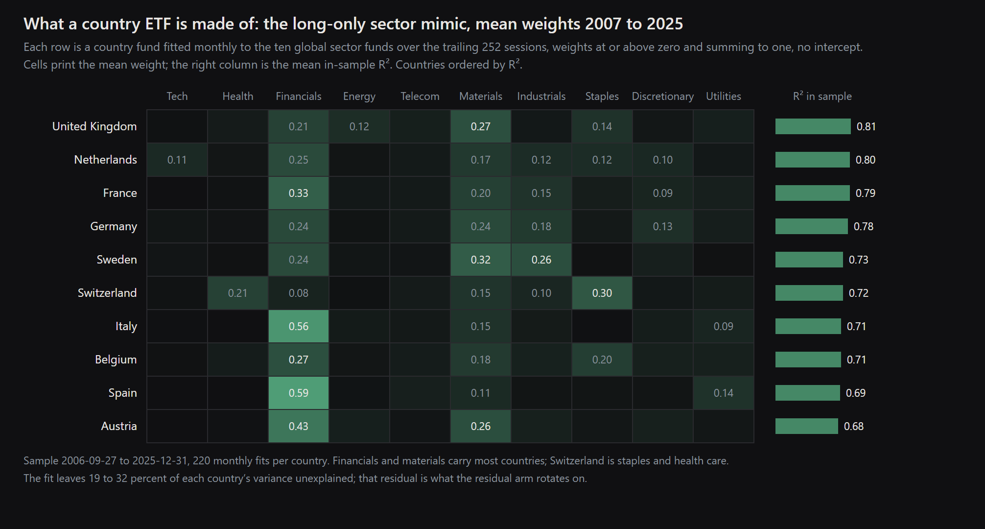
What a country is made of. Across 220 monthly fits the mimic explains 74 percent of a country's daily variance on average, from 68 for Austria to 81 for the United Kingdom; forward, with last month's weights, 71 percent. Financials carry Italy (0.56), Spain (0.59) and Austria (0.43); Switzerland is consumer staples and health care; Sweden is materials and industrials; the United Kingdom is materials and financials. Figure 3 prints the map.
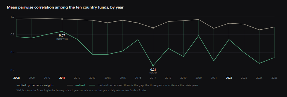
The gap. The sector weights imply a mean pairwise correlation among the countries of 0.93 to 0.99 every year; the realised one ran 0.72 to 0.92. The gap averaged 0.14 and ran from 0.07 in 2011 to 0.21 in 2017: 0.10 in 2008, 0.07 in 2011 and 0.09 in 2022, when everything European fell together and the mimic was nearly right; 0.21 in 2017, 0.20 in 2019 and 0.19 in 2024, when the countries went their own ways. Part of the implied level is the constraint: weights forced non-negative and summing to one on ten global sectors make every country a variant of the same financials-and-materials blend, so the finding is the gap's movement through time, from 0.07 to 0.21, and the level of 0.14 carries the constraint's own overstatement. Figure 2 prints every year.
The arms, ungated, on the 17 shared windows. Sector arm: +11.8, +9.8 and +11.7 percent a year at 3, 6 and 12 months, mean window Sharpe 0.73 to 0.90, mean window drawdown 14 percent, compounded over the seventeen windows to 6.2x, 4.5x and 5.9x. Country arm: +9.1, +10.9 and +10.4, Sharpe 0.57 to 0.67, drawdown 19 percent, 3.2x, 4.3x and 4.0x. Residual arm: +9.9, +11.3 and +9.7, Sharpe 0.63 to 0.67, drawdown 19 percent, 3.7x, 4.5x and 3.6x. The equal-weight ten-country ruler returned +9.7 a year on the same windows and compounded to 3.8x; IEV +8.5 and 3.4x. Two pairs of measures run through this paper and neither pair reconciles. Mean window drawdown is the mean, across windows, of the deepest fall inside each one-year window, while the family table prints each walk's worst drawdown over its whole stitched track, which is deeper. Mean annual return is the average of the one-year window returns, while the CAGR column in that table is the compounded rate, which is why the host cell reads +9.1 a year over eighteen windows in the gate table and 7.9 percent there.
Against the ruler. The sector cells beat holding all ten equally by +2.1, +0.1 and +2.0 a year at 3, 6 and 12 months, standard errors near 3, in 9, 8 and 9 windows of 17; the country cells by -0.6, +1.2 and +0.7 in 6, 7 and 8; the residual cells by +0.2, +1.6 and +0.0 in 9, 9 and 9. No cell in the family, gated or not, beat the ruler in more than 10 windows of 17. Over the seventeen windows compounded, the sector arm at 12 months turned one dollar into 5.95 against 3.83 for the ruler; the same arm over all eighteen windows, 2008 included, 3.90 against 2.04. The family table on this page shows a larger growth against the dispersion-gated sector cell at twelve months than against the host. On the seventeen windows the two share they are the same walk, +11.7 a year each and 5.95 against 5.90 compounded; the difference on the page is the 2008 window, which the gated cell never ran because its threshold needed three years of dispersion history and which cost the host 34.4 points. A growth column is each walk over its own windows and does not rank walks of different lengths. The residual arm was killed by a criterion written before the walk, and the case for the sector arm is not its mean either: the difference from the ruler sits inside one standard error for every arm, and what separates the sector arm is the compounding, the drawdown and the Sharpe. Deflated against the declared family of thirty, the host cell's pooled Sharpe of 0.50 carries a 51 percent probability of being real. The correction is built for the largest draw of a search, and this cell is not it: the highest pooled daily Sharpe in the family is 0.69, on the dispersion-gated sector cell at twelve months, which deflates to 76 percent against the same thirty. Pooled daily Sharpe, the family table and the headline card, is a different statistic from the mean window Sharpe in Tables 1 and 2, and this paragraph names which one it uses each time.
Residual against country, paired on the shared windows. At 3 months the residual ranking added +0.8 a year, standard error 0.61, ahead in 10 of 17 windows; at 6 months +0.3 (0.98, 6 of 17); at 12 months -0.8 (1.04, 10 of 17). Sector against country: +2.7, -1.1 and +1.2 at 3, 6 and 12 months, with standard errors near 4 because the two books hold different instruments; sector against residual +1.9, -1.5 and +2.0. The contrasts that clear a sign test are under the trend gate: sector against residual at 12 months, +3.2 a year in 14 of 17 windows, p 0.01; sector against country there, +2.3 in 13 of 17, p 0.02; and sector against country at 3 months, 12 of 16, p 0.04.
The gates on the shared windows. The trend gate cost every arm at every lookback, 5.6 points a year on average, and led the ungated cell in 1 to 4 windows. Its worst year on the sector arm at twelve months was 2020, when the gate returned -15.7 against +16.4 ungated: it sold after the fall and was in bills for the recovery. The dispersion gate cost 0.7 points a year on average and led in 5 to 9 windows of 17. Raising its threshold to the 70th percentile, rerun at six months only, changed nothing on the country and residual arms, within a point, and added +2.0 on the sector arm, 11 of 15 windows. The registered criterion asked whether the gate works at one threshold only. It does not: it works at neither on two arms and helps one sector cell, so it survives the criterion, and it costs 0.7 points a year to keep.
The trend gate with 2008 in. The shared-window rule removes the one window the gate exists for, so the cells that ran 2008, the country and sector arms, are compared again on all 18. Sector arm at 12 months: ungated +9.1 a year, 3.90x compounded, -34.4 in 2008, worst window drawdown 46 percent; trend-gated +6.5 a year, 2.71x, -6.2 in 2008, worst window drawdown 30 percent, ahead of the ungated cell in 5 windows of 18. Country arm at 12 months: ungated +7.7 and 2.46x with -38.7 in 2008, gated +4.2 and 1.66x with -9.4. The gate bought its protection in 2008 and paid for it in the other seventeen: over eighteen windows it kept 69 percent of the ungated terminal wealth on the sector arm and 67 on the country arm.
The kill criteria, as registered. Reconstruction: the median in-sample R squared is 0.73, above the 0.6 floor; survives. The gap: episodic, 0.07 to 0.21, with its pattern reversed; survives as a finding, with the sign the registration did not expect. The residual arm against holding all ten equally after costs: +0.2, +1.6 and +0.0 a year, ahead in 9, 9 and 9 windows of 17, within one standard error of zero at every lookback; that is not beating the ruler, and the arm is killed by its own criterion. The dispersion gate at one threshold only: it is the same at both thresholds on two arms and helps one sector cell; survives, and costs 0.7 points a year. Break-even trading costs, computed from each cell's own cost ladder as the charge per side at which the arm would only match the ruler: the sector arm 43 basis points at 12 months, 30 at 3 and 11 at 6; the residual arm 29 at 6 months, 12 at 3 and 9 at 12; the country arm 25 at 6 months, 22 at 12 and 5 at 3. A liquid US-listed fund trades at 2 to 5 basis points of spread, so eight of the nine clear that charge, by 4 to 38 basis points. The ninth does not: the country arm at three months breaks even at 4.6 basis points a side, inside the spread itself, and fails the criterion it was registered against. The gated cells' ladders ride their lane, so their break-even is not stated.
2.1 Headline
This paper answers for a declared family of 30 registered studies. 30 member walks are drawn as 30 lines, each chained across its own out-of-sample windows, on one calendar axis, all rebased to 1× on the first session they share. 6 of them are shown to start, the ones the paper reads by; the others are switched off until their name is clicked. The paper’s own walk is the heavy line; the dashed grey line is the study’s own benchmark.
 Open in the lab starts from the heavy line marked with it, this study’s strategy.
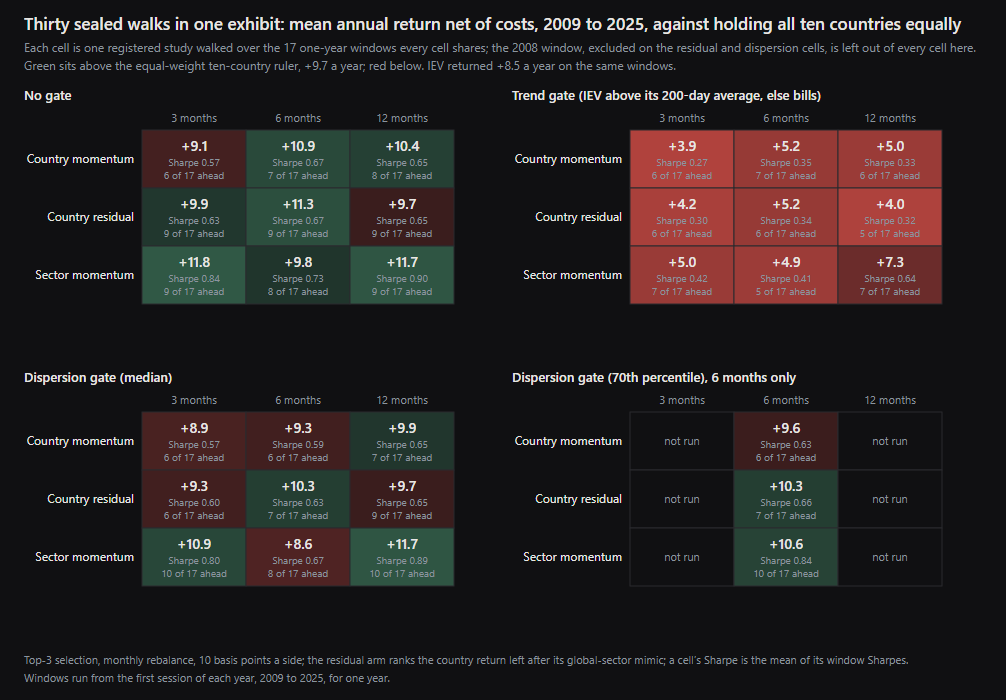
Table 1. Mean annual return net of costs, mean window Sharpe, the count of windows ahead of the equal-weight ten-country ruler, mean window drawdown (the deepest fall inside a window, averaged), and the compounded growth of one dollar, on the 17 windows every cell shares (2009 to 2025). The ruler returned +9.7 a year and compounded to 3.8x; IEV +8.5 and 3.4x. The standard error of each mean across the 17 windows runs 5.2 to 5.3 points a year on the country arm, 4.9 to 5.4 on the residual arm and 2.6 to 2.8 on the sector arm, which is why this paper rests on the ordering and the compounding rather than on a mean.
| Arm | 3 months | 6 months | 12 months |
|---|---|---|---|
| Country momentum | +9.1 0.57 · 6 · -19 · 3.2x | +10.9 0.67 · 7 · -18 · 4.3x | +10.4 0.65 · 8 · -19 · 4.0x |
| Country residual | +9.9 0.63 · 9 · -19 · 3.7x | +11.3 0.67 · 9 · -19 · 4.5x | +9.7 0.65 · 9 · -19 · 3.6x |
| Sector momentum | +11.8 0.84 · 9 · -14 · 6.2x | +9.8 0.73 · 8 · -14 · 4.5x | +11.7 0.90 · 9 · -14 · 5.9x |
Table 2. The same cells under the trend gate (IEV above its 200-day average holds the arm, below it the bill sleeve) and under the dispersion gate at its trailing median (below the median every fund is held equally): mean return, mean window Sharpe, windows ahead of the ruler, mean window drawdown.
| Arm | Trend, 3m | Trend, 6m | Trend, 12m | Dispersion, 3m | Dispersion, 6m | Dispersion, 12m |
|---|---|---|---|---|---|---|
| Country momentum | +3.9 0.27 · 6 · -16 | +5.2 0.35 · 7 · -15 | +5.0 0.33 · 6 · -15 | +8.9 0.57 · 6 · -19 | +9.3 0.59 · 6 · -19 | +9.9 0.65 · 7 · -19 |
| Country residual | +4.2 0.30 · 6 · -15 | +5.2 0.34 · 6 · -15 | +4.0 0.32 · 5 · -15 | +9.3 0.60 · 6 · -19 | +10.3 0.63 · 7 · -19 | +9.7 0.65 · 9 · -19 |
| Sector momentum | +5.0 0.42 · 7 · -12 | +4.9 0.41 · 5 · -12 | +7.3 0.64 · 7 · -11 | +10.9 0.80 · 10 · -14 | +8.6 0.67 · 8 · -14 | +11.7 0.89 · 10 · -13 |
Table 3. Mean difference in annual return, points a year, its standard error across the 17 shared windows, the count of windows the first arm led, and the one-sided sign test on that count. Ungated cells unless the row says otherwise. The mean and its standard error use all 17 windows. The sign test drops the windows in which the two books returned the same figure, which happens whenever a gate did not fire and, in two windows of the ungated sector-minus-country row at twelve months, because two different books landed on the same return to the tenth of a point the ledger keeps. A denominator below 17 is the count of windows in which the two differed at that precision.
| Contrast | 3 months | 6 months | 12 months |
|---|---|---|---|
| Residual minus country | +0.81 (0.61), 10 of 17, p 0.31 | +0.34 (0.98), 6 of 17, p 0.93 | -0.77 (1.04), 10 of 17, p 0.31 |
| Sector minus country | +2.71 (3.78), 10 of 17, p 0.31 | -1.14 (4.10), 9 of 17, p 0.50 | +1.23 (3.87), 8 of 15, p 0.50 |
| Sector minus residual | +1.90 (3.65), 9 of 17, p 0.50 | -1.48 (4.05), 8 of 17, p 0.69 | +2.00 (3.43), 11 of 17, p 0.17 |
| Sector minus country, trend gate | +1.13 (2.73), 12 of 16, p 0.04 | -0.30 (3.31), 10 of 17, p 0.31 | +2.25 (2.95), 13 of 17, p 0.02 |
| Sector minus residual, trend gate | +0.79 (2.56), 9 of 17, p 0.50 | -0.32 (3.11), 10 of 17, p 0.31 | +3.25 (2.54), 14 of 17, p 0.01 |
Table 4. Gated minus ungated on the shared windows, points a year with the standard error and the count of windows the gate led, at each lookback; the last column is the 70th-percentile dispersion threshold against the median at six months. As in Table 3 the mean uses all 17 windows and the count drops the windows in which the gated and ungated books returned identically, which is what a gate that did not fire produces.
| Arm | Trend, 3m | Trend, 6m | Trend, 12m | Dispersion, 3m | Dispersion, 6m | Dispersion, 12m | 70th vs median, 6m |
|---|---|---|---|---|---|---|---|
| Country momentum | -5.2 (3.1), 4 of 13 | -5.8 (3.0), 3 of 13 | -5.4 (3.1), 4 of 13 | -0.2 (0.7), 9 of 17 | -1.6 (0.7), 5 of 17 | -0.5 (1.0), 6 of 15 | +0.3 (0.8), 12 of 16 |
| Country residual | -5.7 (3.1), 3 of 13 | -6.1 (3.1), 3 of 13 | -5.6 (2.9), 3 of 13 | -0.6 (0.9), 8 of 17 | -1.0 (0.9), 5 of 16 | +0.0 (0.7), 5 of 14 | +0.0 (0.5), 9 of 15 |
| Sector momentum | -6.8 (2.2), 1 of 13 | -4.9 (2.5), 4 of 14 | -4.4 (2.4), 4 of 14 | -1.0 (1.0), 6 of 17 | -1.2 (0.8), 6 of 17 | +0.0 (1.3), 7 of 17 | +2.0 (0.8), 11 of 15 |
Table 5. The cells that ran 2008, the country and sector arms: mean annual return, compounded growth of one dollar over the eighteen windows, the 2008 window, the worst window drawdown, and the count of windows the gate led. The ruler compounded to 2.0x over the same eighteen windows, +6.6 a year. The last column is the single window in which the gate cost the most, with the gated return against the ungated one.
| Cell | Ungated: mean / growth / 2008 / worst drawdown | Trend-gated: mean / growth / 2008 / worst drawdo | Gate ahead | Gate: worst window |
|---|---|---|---|---|
| Country momentum, 3 months | +6.2 1.75x · -44.6 · -57 | +3.1 1.35x · -10.2 · -37 | 5 of 18 | 2020: -20.9 vs +17.1 |
| Country momentum, 6 months | +7.8 2.34x · -46.0 · -58 | +4.4 1.66x · -9.1 · -37 | 4 of 18 | 2020: -23.5 vs +13.1 |
| Country momentum, 12 months | +7.7 2.46x · -38.7 · -54 | +4.2 1.66x · -9.4 · -34 | 5 of 18 | 2020: -20.8 vs +16.4 |
| Sector momentum, 3 months | +9.1 3.88x · -37.6 · -48 | +4.4 1.99x · -5.8 · -29 | 2 of 18 | 2020: -13.3 vs +20.8 |
| Sector momentum, 6 months | +7.3 2.91x · -34.8 · -45 | +4.2 1.92x · -6.3 · -29 | 5 of 18 | 2020: -8.1 vs +30.1 |
| Sector momentum, 12 months | +9.1 3.90x · -34.4 · -46 | +6.5 2.71x · -6.2 · -30 | 5 of 18 | 2020: -15.7 vs +16.4 |
Table 6. For each ungated cell on the shared windows: mean annual return before trading costs and after the 10 basis points a side charged, the cost bill that charge produced, and the charge per side at which the arm would only match the equal-weight ruler (below zero where the cell trails the ruler before any charge). Fund fees are the expense ratios read from the fund data on 2026-09-07 and are inside every return in this paper. The net column is the same quantity as the mean annual return in Table 1: both are measured against the uncharged capital the window opened with, and the two tables agree to a hundredth of a point on every cell.
| Cell | Gross, a year | Net, a year | Cost bill at 10 bps | Break-even, bps a side | Fund fee, a year |
|---|---|---|---|---|---|
| Country momentum, 3 months | +10.17 | +9.15 | 1.02 | 4.6 | 0.50 |
| Country momentum, 6 months | +11.77 | +10.95 | 0.82 | 25.1 | 0.50 |
| Country momentum, 12 months | +11.05 | +10.42 | 0.62 | 21.6 | 0.50 |
| Country residual, 3 months | +11.03 | +9.95 | 1.08 | 12.3 | 0.50 |
| Country residual, 6 months | +12.09 | +11.27 | 0.81 | 29.3 | 0.50 |
| Country residual, 12 months | +10.27 | +9.66 | 0.62 | 9.3 | 0.50 |
| Sector momentum, 3 months | +12.94 | +11.84 | 1.10 | 29.5 | 0.37 |
| Sector momentum, 6 months | +10.56 | +9.80 | 0.76 | 11.4 | 0.37 |
| Sector momentum, 12 months | +12.25 | +11.65 | 0.60 | 42.7 | 0.37 |
Table 7. The mimic per country over 220 monthly fits: mean in-sample R squared, mean forward R squared, and the two sectors with the largest mean weight. Weights are long-only and sum to one.
| Country | R squared in sample | R squared forward | Largest weight | Second weight |
|---|---|---|---|---|
| The United Kingdom | 0.81 | 0.78 | Materials 0.27 | Financials 0.21 |
| The Netherlands | 0.80 | 0.78 | Financials 0.25 | Materials 0.17 |
| France | 0.79 | 0.77 | Financials 0.33 | Materials 0.20 |
| Germany | 0.78 | 0.75 | Financials 0.24 | Materials 0.24 |
| Sweden | 0.73 | 0.71 | Materials 0.32 | Industrials 0.26 |
| Switzerland | 0.72 | 0.70 | Consumer staples 0.30 | Health care 0.21 |
| Italy | 0.71 | 0.68 | Financials 0.56 | Materials 0.15 |
| Belgium | 0.71 | 0.67 | Financials 0.27 | Consumer staples 0.20 |
| Spain | 0.69 | 0.66 | Financials 0.59 | Utilities 0.14 |
| Austria | 0.68 | 0.64 | Financials 0.43 | Materials 0.26 |
Table 8. Total return over each one-year window, percent, on the walk's own sessions (first session of January to the last of December): IEV, the equal-weight ten-country book rebalanced monthly, and SPY; two windows per row. Every arm is measured against the second.
| Window | IEV | Ten countries | SPY | Window | IEV | Ten countries | SPY |
|---|---|---|---|---|---|---|---|
| 2008 | -43.2 | -46.7 | -36.8 | 2009 | +27.6 | +33.9 | +26.4 |
| 2010 | +1.0 | +2.6 | +15.1 | 2011 | -12.1 | -16.8 | +1.9 |
| 2012 | +16.9 | +19.4 | +16.0 | 2013 | +22.4 | +22.9 | +32.3 |
| 2014 | -5.1 | -6.4 | +13.5 | 2015 | -2.8 | -0.6 | +1.2 |
| 2016 | +1.9 | +3.2 | +13.6 | 2017 | +24.6 | +28.1 | +21.7 |
| 2018 | -15.2 | -16.7 | -4.6 | 2019 | +24.7 | +24.1 | +31.2 |
| 2020 | +3.2 | +4.1 | +18.4 | 2021 | +15.5 | +15.6 | +28.7 |
| 2022 | -15.0 | -17.2 | -18.2 | 2023 | +18.4 | +19.9 | +26.2 |
| 2024 | +2.6 | +4.0 | +24.9 | 2025 | +36.1 | +44.9 | +17.7 |
2.2 Per-step results
| # | Step | Out-of-sample window | Sharpe |
|---|---|---|---|
| 1 | Euro rotation · sector · 12m · none · step 1 | 2008-01-02 → 2008-12-31 | -0.92 |
| 2 | Euro rotation · sector · 12m · none · step 2 | 2009-01-02 → 2009-12-31 | 0.75 |
| 3 | Euro rotation · sector · 12m · none · step 3 | 2010-01-04 → 2010-12-31 | 0.55 |
| 4 | Euro rotation · sector · 12m · none · step 4 | 2011-01-03 → 2011-12-30 | -0.18 |
| 5 | Euro rotation · sector · 12m · none · step 5 | 2012-01-03 → 2012-12-31 | 1.23 |
| 6 | Euro rotation · sector · 12m · none · step 6 | 2013-01-02 → 2013-12-31 | 2.23 |
| 7 | Euro rotation · sector · 12m · none · step 7 | 2014-01-02 → 2014-12-31 | 0.72 |
| 8 | Euro rotation · sector · 12m · none · step 8 | 2015-01-02 → 2015-12-31 | 0.04 |
| 9 | Euro rotation · sector · 12m · none · step 9 | 2016-01-04 → 2016-12-30 | 0.29 |
| 10 | Euro rotation · sector · 12m · none · step 10 | 2017-01-03 → 2017-12-29 | 2.48 |
| 11 | Euro rotation · sector · 12m · none · step 11 | 2018-01-02 → 2018-12-31 | -0.53 |
| 12 | Euro rotation · sector · 12m · none · step 12 | 2019-01-02 → 2019-12-31 | 1.97 |
| 13 | Euro rotation · sector · 12m · none · step 13 | 2020-01-02 → 2020-12-31 | 0.64 |
| 14 | Euro rotation · sector · 12m · none · step 14 | 2021-01-04 → 2021-12-31 | 1.26 |
| 15 | Euro rotation · sector · 12m · none · step 15 | 2022-01-03 → 2022-12-30 | 0.16 |
| 16 | Euro rotation · sector · 12m · none · step 16 | 2023-01-03 → 2023-12-29 | 0.56 |
| 17 | Euro rotation · sector · 12m · none · step 17 | 2024-01-02 → 2024-12-31 | 1.72 |
| 18 | Euro rotation · sector · 12m · none · step 18 | 2025-01-02 → 2025-12-31 | 1.37 |
2.2b The family, walk by walk
Figure 4 draws these walks; here is every one of them in numbers, the paper’s own walk first and the study’s benchmark last.
| Walk | Windows | Span | Growth | CAGR | Worst drawdown | Pooled Sharpe |
|---|---|---|---|---|---|---|
| sector · 12m · none (this paper, the one the lab opens) | 18 | 2008-01-02 → 2025-12-31 | +290.4% | +7.9% | -53.4% | 0.50 |
| country · 12m · dispersion | 18 | 2008-01-02 → 2025-12-31 | +112.2% | +4.3% | -62.7% | 0.30 |
| country · 12m · none | 18 | 2008-01-02 → 2025-12-31 | +145.6% | +5.1% | -58.9% | 0.34 |
| country · 12m · trend | 18 | 2008-01-02 → 2025-12-31 | +65.7% | +2.8% | -38.0% | 0.26 |
| country · 3m · dispersion | 18 | 2008-01-02 → 2025-12-31 | +77.4% | +3.2% | -63.0% | 0.25 |
| country · 3m · none | 18 | 2008-01-02 → 2025-12-31 | +75.7% | +3.2% | -62.6% | 0.26 |
| country · 3m · trend | 18 | 2008-01-02 → 2025-12-31 | +35.1% | +1.7% | -45.3% | 0.18 |
| country · 6m · dispersion | 18 | 2008-01-02 → 2025-12-31 | +83.6% | +3.4% | -63.7% | 0.26 |
| country · 6m · dispersion70 | 18 | 2008-01-02 → 2025-12-31 | +97.2% | +3.8% | -63.4% | 0.28 |
| country · 6m · none | 18 | 2008-01-02 → 2025-12-31 | +134.1% | +4.8% | -63.7% | 0.33 |
| country · 6m · trend | 18 | 2008-01-02 → 2025-12-31 | +66.3% | +2.9% | -41.4% | 0.26 |
| residual · 12m · dispersion | 17 (1 excluded) | 2009-01-02 → 2025-12-31 | +274.1% | +8.1% | -42.3% | 0.46 |
| residual · 12m · none | 17 (1 excluded) | 2009-01-02 → 2025-12-31 | +263.4% | +7.9% | -39.2% | 0.46 |
| residual · 12m · trend | 17 (1 excluded) | 2009-01-02 → 2025-12-31 | +55.8% | +2.6% | -41.7% | 0.24 |
| residual · 3m · dispersion | 17 (1 excluded) | 2009-01-02 → 2025-12-31 | +250.0% | +7.7% | -37.6% | 0.45 |
| residual · 3m · none | 17 (1 excluded) | 2009-01-02 → 2025-12-31 | +266.7% | +7.9% | -37.6% | 0.46 |
| residual · 3m · trend | 17 (1 excluded) | 2009-01-02 → 2025-12-31 | +61.9% | +2.9% | -43.2% | 0.26 |
| residual · 6m · dispersion | 17 (1 excluded) | 2009-01-02 → 2025-12-31 | +292.5% | +8.4% | -43.1% | 0.48 |
| residual · 6m · dispersion70 | 17 (1 excluded) | 2009-01-02 → 2025-12-31 | +304.4% | +8.6% | -41.6% | 0.48 |
| residual · 6m · none | 17 (1 excluded) | 2009-01-02 → 2025-12-31 | +345.7% | +9.2% | -40.6% | 0.52 |
| residual · 6m · trend | 17 (1 excluded) | 2009-01-02 → 2025-12-31 | +86.4% | +3.7% | -43.3% | 0.30 |
| sector · 12m · dispersion | 17 (1 excluded) | 2009-01-02 → 2025-12-31 | +490.1% | +11.0% | -30.3% | 0.69 |
| sector · 12m · trend | 18 | 2008-01-02 → 2025-12-31 | +170.2% | +5.7% | -30.0% | 0.48 |
| sector · 3m · dispersion | 17 (1 excluded) | 2009-01-02 → 2025-12-31 | +415.0% | +10.1% | -30.4% | 0.64 |
| sector · 3m · none | 18 | 2008-01-02 → 2025-12-31 | +287.9% | +7.8% | -52.7% | 0.50 |
| sector · 3m · trend | 18 | 2008-01-02 → 2025-12-31 | +98.6% | +3.9% | -29.2% | 0.35 |
| sector · 6m · dispersion | 17 (1 excluded) | 2009-01-02 → 2025-12-31 | +269.5% | +8.0% | -30.7% | 0.53 |
| sector · 6m · dispersion70 | 17 (1 excluded) | 2009-01-02 → 2025-12-31 | +399.2% | +9.9% | -30.7% | 0.64 |
| sector · 6m · none | 18 | 2008-01-02 → 2025-12-31 | +191.2% | +6.1% | -50.7% | 0.41 |
| sector · 6m · trend | 18 | 2008-01-02 → 2025-12-31 | +92.0% | +3.7% | -28.7% | 0.34 |
| Ten countries held equally, rebalanced monthly, total return (benchmark) | 2008-01-02 → 2025-12-31 | +103.1% | +4.0% | -64.0% |
Growth and CAGR above are each walk over its own windows, so they are not comparable across walks with different window counts: a walk that excluded a window did not live through it. The figure rebases every line on the session all of them share.
2.3 Search accounting
This paper's search is a declared family: the European country rotation grid, one pre-registered design: ten single-country ETFs rotated monthly by trailing momentum on three arms, the country itself, the country residual after its global-sector mimic, and the global sectors themselves, at three lookbacks and under three gates, none, a trend gate on the European market, and a dispersion gate, plus the three arms at six months with the dispersion threshold raised to its 70th percentile, 30 sealed studies in all, every one reported, counted at N = 30 evaluated books. Every member is either a registered walk with its own hypothesis and frozen record, or a derived average computed from those frozen records; every member is reported, in the family figure and table, and none was selected away. The count is declared by the author rather than derived from one project's ledger, because the members are sibling registered studies; the declaration names them and is frozen in this artifact. A conservative deflated-Sharpe adjustment for this N appears once, in Appendix A. What the source strategy's author searched before publishing is not knowable from here and is not counted. The registered per-step record below still guarantees each window's hypothesis was hashed and registered before that window was scored.
3 The circuit
The strategy is a circuit of platform primitives, frozen when the study is registered. Below is the circuit as wired on the canvas, the objective it encodes and how the search runs through it, followed by the mathematics each primitive actually computes, the same formulas the execution engine runs. The complete parameterisation is preserved in the study ledger (Appendix A).
The sentence below is the registration record, generated when the circuit was registered and printed verbatim; the authored description of the design is Section 1.
A configured universe, selected by statistical / factor criteria, rebalanced monthly across the selected basket, and run out-of-sample from the anchor: anything the design estimates from history, where it estimates at all, is re-estimated at each anchor from pre-anchor data only, and the walk advances through registered out-of-sample windows; its disposition is the realized forward path versus the benchmark, is expected to generate positive risk-adjusted returns over the forward test window.
This is the host cell of the family: the sector arm at twelve months, ungated, the simplest machine of the thirty and the one every headline number on this page comes from. It ranks the ten global sector funds on their trailing twelve-month return, buys the top three equally and rebalances monthly. It carries neither primitive written for this study, because ranking the sectors themselves needs neither. The registration sentence above is the platform record for this shape of circuit and names no instrument; the design is Section 1. The sector mimic and the dispersion gate are sealed in the cells that use them, and the figure after the diagram prints one of those cells.
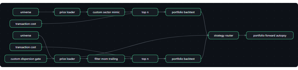
Envelopes show counts, ratios, dates, and the parameters the author chose. Full price and per-name data series are not republished: the underlying market data is licensed to QuanterLab. Point figures quoted in the prose, a named holding's return over a stated span, are summary facts derived from public market prices, not redistributed series.
The objective and the search
| Universe | European rotation books (fixed lists), named fixed instrument lists, no membership reconstruction applies: sectors {IXN, IXJ, IXG, IXC, IXP, MXI, EXI, KXI, RXI, JXI}. |
|---|---|
| Selection | metric across mom_trailing → highest 3 kept by mom_trailing. |
| Validation & out-of-sample | portfolio forward test (buy-and-hold book) (1y horizon from the anchor, monthly rebalance); overlays: Transaction Cost. |
| Other components | Forward-test autopsy: Portfolio Forward Autopsy. |
Cost elements are wired into the circuit, the realised drag is reported per step in Appendix B.
Show the mathematics, 5 primitives, formulas and parity notes
3.1 Price Loader
Bulk OHLCV fetch for the whole universe, point-in-time, no future bars.
Momentum, volatility, trend, every price-based metric needs history. This loads open/high/low/close/volume for all names in parallel, clipped so nothing after the anchor can leak in. The lookback window is derived automatically from the deepest metric you wired.
It loads exactly enough history for the hungriest downstream metric plus a warm-up buffer:
W = \max_k(\text{lookback}_k) + \text{buffer}, \qquad \text{bars} \le \text{anchor } t3.2 Top N
Keep the best N, rank, then cut.
Sort the survivors by the Composite Σ (or, if none is wired, the last metric in the chain) and keep the top (or bottom) N. The final narrowing from a scored list to a committed basket.
\text{Top-}N = \{\, i : \operatorname{rank}(\text{score}_i) \le N \,\}N = \operatorname{round}(f \cdot n_{\text{ranked}})\text{kept} = \{\, i \in H : \operatorname{rank}_i \le K \,\} \;\cup\; \text{best ranked } i \notin H \text{ up to } N3.3 Portfolio Backtest
Replay the portfolio forward, rebalanced, point-in-time, with costs.
Holds the basket and rebalances on schedule, re-selecting and re-optimizing point-in-time at each rebalance (so it only ever uses information available then), and reports the equity curve, Sharpe, drawdown and trade stats, optionally net of cost and risk overlays.
E_t = E_{t-1}\big(1 + \mathbf w_{t}^{\top}\mathbf r_t - \text{costs}_t\big)\text{DD}_t = \frac{E_t}{\max_{\tau\le t}E_\tau} - 1, \qquad \text{MaxDD} = \min_t \text{DD}_t\text{charge}_t \;=\; \text{loan}_t \cdot \frac{\text{spread}}{252}, \qquad \text{loan}_t = \begin{cases}\max(0,\,-\text{cash}_t) & \text{institutional (netted)}\\ \max(0,\,\text{long MV}_t - E_t) & \text{retail (no netting)}\end{cases}\mathbf w_k = \{\, w_{k,i} : i \in \text{held} \,\}, \qquad \text{cash}_k = 1 - \textstyle\sum_{i \in \text{held}} w_{k,i}3.4 Transaction Cost
Charge for trading, slippage + commission on every turn.
Real trading isn't free. This deducts a cost proportional to how much you trade (turnover), in basis points, so the backtest reflects net, not gross, performance.
\text{cost}_t = \frac{\text{bps}}{10{,}000}\;\times\;\text{turnover}_t, \qquad \text{turnover}_t = \tfrac12\sum_i \lvert w_{i,t}-w_{i,t^-}\rvert3.5 Portfolio Forward Autopsy
The post-mortem, where the forward test’s return actually came from.
Runs after the Portfolio Forward Test and dissects its realized path: per-rebalance contributions, winners and losers, exposure and cash periods, and how the realized route compares to what the risk cones projected. It computes nothing new about the future, it explains the past the book just lived.
Depth I–IV: headline attribution, per-segment breakdown, per-name contributions, and the calibration ledger (projected cone vs realized, segment by segment). In a study, this is the node that fills the appendices.
4 Projection calibration, pooled across the walk
Every rebalance carried a Monte Carlo cone and a 95% VaR estimated before the segment it is scored against. Two questions, pooled over the whole study: did realized outcomes land inside the band as often as the band claims, and were VaR breaches as frequent as 5%?
This section is produced by the forward tester itself: every portfolio backtest fits the cone and the VaR estimate at each rebalance and scores them against the segment that followed. It does not require, and this circuit does not contain, a Monte Carlo primitive; that primitive is a separate, standalone analysis.
| Arm | Steps | Rebalances | In band | Coverage | Expected | VaR days | Breach rate | Expected |
|---|---|---|---|---|---|---|---|---|
| Portfolio | 18 | 229 | 197 / 216 | 91.2% ±1.93 | 90.0% | 4313 | 5.24% ±0.339 | 5.0% |
± values are binomial standard errors on the estimate. A coverage figure below the expected band means the projection was over-confident; a breach rate above 5% means the same of the risk model. Both forecasts used only data prior to the segment scored.
5 Discussion
5.1 Interpretation
The answer to the question as registered is yes, mostly. A European country fund is three-quarters a long-only sector portfolio, and the quarter it is not does not pay to rotate on. The sector arm returned more than the country arm at 3 and 12 months and less at 6, with the standard error near 4 points a year at all three. What separates them is the drawdown and the Sharpe, and that ordering holds at every lookback: ten global sector funds are a wider and less correlated set than ten European country funds that share the same banks and the same currency. Over eighteen windows the difference compounds to 3.9x against 2.5x. The wrapper does not explain it: the sector funds charge 0.13 points a year less than the country funds, against arm differences of +2.7, -1.1 and +1.2 at the three lookbacks.
The mimic leaves 19 to 32 percent of each country's variance unexplained, and the correlation gap says the unexplained part moves countries apart rather than together, by 0.07 to 0.21 of correlation a year. It is largest in the calm years, when a country can go its own way, and smallest in 2008, 2011 and 2022, when everything European fell as one. That is a fact about diversification. What a country adds to a European book is there in the years a reader does not need it. The residual has no trailing-return signal worth a top-three book. Ranking on it added +0.8 points a year over the raw country ranking at 3 months and +0.3 at 6, and lost +0.8 at twelve.
Heston and Rouwenhorst (1994) found country effects dominating industry effects in European returns; Cavaglia, Brightman and Aked (2000) found industry factors overtaking country factors by the late 1990s; Bekaert, Hodrick and Zhang (2009) found the country factor alive in comovement. This walk is on the tradeable version of the question, ten funds a retail investor can hold, and reads as the middle paper: the sectors explain most of a country, the rest is real, and only the first part is a rotation.
The risk engine, graded. Before every rebalance the forward tester fits a Monte Carlo cone and a 95 percent VaR on data before the segment it then scores. Over the host walk 197 of 216 cones contained the outcome, 91 percent against a 90 percent claim, and the VaR was breached on 5.24 percent of 4,313 days against 5 expected, each within one standard error of its claim over eighteen years.
Two primitives were written for this study and sit in the Custom group of the platform's palette, where any later study can wire them: the sector mimic, a stockset-to-stockset node that fits the countries to the sectors as of the anchor and hands the forward residual momentum down as the ranking metric, and the dispersion gate, a regime node the router reads. Their behaviour was pinned by tests before the walk: a synthetic country built from two sectors is recovered exactly with a forward R squared of one, the gate labels a hand-built calm panel and a hand-built stressed panel the right way round, and the monthly label holds between month-ends. Every cell is a sealed study on this platform with its 18 windows, its registered claim and its per-step record; the fit tables and the gap series are computed once from the same loader and frozen with the paper.
The residual is largest where the mimic fits worst, Austria at 0.68 and Spain at 0.69. The second tier of country funds that list from 2010 and 2012 is smaller and less bank-heavy still, and that is the next walk.
This study is one member of a declared search family: the same design walked at several settings across sibling registered projects, every member either a registered walk with its own frozen record or a derived average of those records, and every member reported. The family size is declared by the author and named in the lineage; it is the search-accounting count for this paper. What was searched before the source strategy was published is not knowable from here and is not counted.
5.2 Limitations
Ten countries and ten sectors, in dollars: a country's residual includes its currency against the dollar, and a euro-based reader would see a different residual. The second tier of country funds was kept out of the arms by its listing dates.
Seventeen shared windows are few. The standard error of each arm mean, printed in the caption of Table 1, runs 4.9 to 5.4 points a year on the country and residual arms and 2.6 to 2.8 on the sector arm; the paper's claims rest on the drawdown and Sharpe ordering, which holds at every lookback, on the compounding, and on the residual arm's failure to beat the equal-weight ruler. Deflated against thirty cells, the host's pooled Sharpe has a 51 percent probability of being real, and the family's highest, 0.69 on the dispersion-gated sector cell at twelve months, deflates to 76 percent; the reader should carry that number, not the raw Sharpe.
The ten residual cells and the four dispersion-gated sector cells have no 2008 window, so their compounding runs over seventeen windows and their lines on the family figure start in 2009; the figure rebases every line on the first session all of them share, and the family table prints each walk over its own windows with the exclusion counted. A residual cell's compounding is compared with the others on the shared windows only.
Costs are 10 basis points a side; break-even costs are stated for the ungated cells, whose cost ladder is the book's own, and withheld for the gated cells. The implied correlation the mimic reports is partly the long-only constraint's doing, so the level of the gap is overstated and only its movement through time is read. The European rulers were computed outside the engine from the same loader on the walk's own sessions and are total return.
The dispersion gate decides at month-ends and its threshold uses a trailing window of three years; the trend gate's bill sleeve is one fund. Neither gate was tuned; the trend gate cost 5.6 points a year on the shared windows and bought its protection in 2008 alone.
References
- Bailey, D. H., & López de Prado, M. (2014). The Deflated Sharpe Ratio: Correcting for Selection Bias, Backtest Overfitting, and Non-Normality. Journal of Portfolio Management, 40(5), 94–107. doi:10.3905/jpm.2014.40.5.094
- Heston, S. L. and Rouwenhorst, K. G. (1994). Does industrial structure explain the benefits of international diversification? Journal of Financial Economics, 36(1), 3 to 27. Country effects dominated industry effects in twelve European markets, 1978 to 1992.
- Cavaglia, S., Brightman, C. and Aked, M. (2000). The increasing importance of industry factors. Financial Analysts Journal, 56(5), 41 to 54. Industry factors overtook country factors in developed-market returns during the late 1990s.
- Bekaert, G., Hodrick, R. J. and Zhang, X. (2009). International stock return comovements. The Journal of Finance, 64(6), 2591 to 2626. A country factor remains in the comovement of developed-market returns after industry factors.
- Asness, C. S., Moskowitz, T. J. and Pedersen, L. H. (2013). Value and momentum everywhere. The Journal of Finance, 68(3), 929 to 985. Momentum in country equity indices, among other asset classes, with the rankings the country arm here uses.
Appendix A Reproducibility in QuanterLab
Conservative upper-bound adjustment. Deflating the pooled Sharpe of 0.50 for the declared family count of N = 30 gives a 51% probability that the result is genuinely positive rather than the best of N noisy draws (Bailey & López de Prado, 2014), the strategy does not clear the multiple-testing correction on its own pooled Sharpe. Registered candidates are heavily correlated (near-identical variants), so this deflation is an upper bound on the multiple-testing penalty, not a precise correction; the raw count in §2.3 is the primary artifact. The correction is built for the LARGEST draw of a search, and this cell is not it: the highest pooled Sharpe in the declared family is 0.69, on sector · 12m · dispersion, whose own page carries its own adjustment. Read this number as the penalty for the cell in front of you, not as the penalty for the best of the family.
Each step is backed by a frozen run report. The study is re-derivable from the ledger below.
| # | Commit | Report | Anchor | OOS window |
|---|---|---|---|---|
| 1 | 11ce6ed543b1 | 8525 | 2008-01-01 | 2008-01-02 → 2008-12-31 |
| 2 | 078e179d6eac | 8526 | 2009-01-01 | 2009-01-02 → 2009-12-31 |
| 3 | eb64dc912e12 | 8527 | 2010-01-01 | 2010-01-04 → 2010-12-31 |
| 4 | 7f75683a2ca1 | 8528 | 2011-01-01 | 2011-01-03 → 2011-12-30 |
| 5 | 6d2bb7bb813e | 8529 | 2012-01-01 | 2012-01-03 → 2012-12-31 |
| 6 | 960405aea6d7 | 8530 | 2013-01-01 | 2013-01-02 → 2013-12-31 |
| 7 | b5ef0381fc45 | 8531 | 2014-01-01 | 2014-01-02 → 2014-12-31 |
| 8 | 8df59bbb1131 | 8532 | 2015-01-01 | 2015-01-02 → 2015-12-31 |
| 9 | 388d394d7735 | 8533 | 2016-01-01 | 2016-01-04 → 2016-12-30 |
| 10 | a6162e7e0b3c | 8534 | 2017-01-01 | 2017-01-03 → 2017-12-29 |
| 11 | 385fba0a2db3 | 8535 | 2018-01-01 | 2018-01-02 → 2018-12-31 |
| 12 | 3dba17fb5610 | 8536 | 2019-01-01 | 2019-01-02 → 2019-12-31 |
| 13 | 61f0efca6aff | 8537 | 2020-01-01 | 2020-01-02 → 2020-12-31 |
| 14 | 896440ea4bc3 | 8538 | 2021-01-01 | 2021-01-04 → 2021-12-31 |
| 15 | e23f64d7fec8 | 8539 | 2022-01-01 | 2022-01-03 → 2022-12-30 |
| 16 | 318650ebb521 | 8540 | 2023-01-01 | 2023-01-03 → 2023-12-29 |
| 17 | 9a0038083827 | 8541 | 2024-01-01 | 2024-01-02 → 2024-12-31 |
| 18 | b46088d19a2b | 8542 | 2025-01-01 | 2025-01-02 → 2025-12-31 |
The methods the platform implements, for every study made on it, rest on these works.
- Bailey, D. H., & López de Prado, M. (2014). The Deflated Sharpe Ratio: Correcting for Selection Bias, Backtest Overfitting, and Non-Normality. Journal of Portfolio Management, 40(5), 94–107. doi:10.3905/jpm.2014.40.5.094
- Gelman, A., & Loken, E. (2013). The garden of forking paths: Why multiple comparisons can be a problem, even when there is no “fishing expedition.” Working paper, Columbia University.
- Harvey, C. R., Liu, Y., & Zhu, H. (2016). … and the Cross-Section of Expected Returns. Review of Financial Studies, 29(1), 5–68. doi:10.1093/rfs/hhv059
- Lo, A. W. (2002). The Statistics of Sharpe Ratios. Financial Analysts Journal, 58(4), 36–52. doi:10.2469/faj.v58.n4.2453
Appendix A2 Registration record
What this record does and does not establish. Every window in this study is historical: the data existed before the study began, so this is sequential registration on past windows, not pre-registration in the clinical-trial sense, and no procedure could make it so. What the platform does enforce is order, each step's specification was frozen and hashed before that step was scored, and the walk cannot advance past a step that was never run or close one with a result registered for a different window. The two timestamp columns below are the evidence: read them together and each registration precedes its own run, and each run precedes the next registration. A study whose registrations all post-date its runs would show it here. Wall-clock spacing between registrations varies with the author's schedule and queue latency; the ordering, not the tempo, is the claim.
“A configured universe, selected by statistical / factor criteria, rebalanced monthly across the selected basket, and run out-of-sample from the anchor: anything the design estimates from history, where it estimates at all, is re-estimated at each anchor from pre-anchor data only, and the walk advances through registered out-of-sample windows; its disposition is the realized forward path versus the benchmark, is expected to generate positive risk-adjusted returns over the forward test window.”
The same hypothesis was registered independently at every step, hashed before each step's out-of-sample window was scored:
| # | Anchor | Registered at (UTC) | Run completed (UTC) |
|---|---|---|---|
| 1 | 2008-01-01 | 2026-09-06 20:24:01 | 2026-09-06 20:24:16 |
| 2 | 2009-01-01 | 2026-09-06 20:24:17 | 2026-09-06 20:24:32 |
| 3 | 2010-01-01 | 2026-09-06 20:24:32 | 2026-09-06 20:24:47 |
| 4 | 2011-01-01 | 2026-09-06 20:24:47 | 2026-09-06 20:25:02 |
| 5 | 2012-01-01 | 2026-09-06 20:25:02 | 2026-09-06 20:25:17 |
| 6 | 2013-01-01 | 2026-09-06 20:25:17 | 2026-09-06 20:25:32 |
| 7 | 2014-01-01 | 2026-09-06 20:25:32 | 2026-09-06 20:25:47 |
| 8 | 2015-01-01 | 2026-09-06 20:25:47 | 2026-09-06 20:26:02 |
| 9 | 2016-01-01 | 2026-09-06 20:26:02 | 2026-09-06 20:26:17 |
| 10 | 2017-01-01 | 2026-09-06 20:26:18 | 2026-09-06 20:26:33 |
| 11 | 2018-01-01 | 2026-09-06 20:26:33 | 2026-09-06 20:26:48 |
| 12 | 2019-01-01 | 2026-09-06 20:26:48 | 2026-09-06 20:27:03 |
| 13 | 2020-01-01 | 2026-09-06 20:27:03 | 2026-09-06 20:27:18 |
| 14 | 2021-01-01 | 2026-09-06 20:27:18 | 2026-09-06 20:27:33 |
| 15 | 2022-01-01 | 2026-09-06 20:27:33 | 2026-09-06 20:27:48 |
| 16 | 2023-01-01 | 2026-09-06 20:27:48 | 2026-09-06 20:28:03 |
| 17 | 2024-01-01 | 2026-09-06 20:28:03 | 2026-09-06 20:28:18 |
| 18 | 2025-01-01 | 2026-09-06 20:28:19 | 2026-09-06 20:28:34 |
Appendix B Per-step diagnostics
Realized in the projection tables below is the risk engine scoring its own forecast: the buy-and-hold return of the segment that followed each rebalance, on the same gross basis the cone was projected on. It is deliberately not the charged, calendar-window total return the study’s tables print, so the two will not reconcile line by line; the cone and its outcome share one basis, which is what a calibration test requires. Each row names its segment’s span so a boundary session is visible.
Names held is the union across the window: the count of distinct instruments the book touched between the window’s first and last session, not the number it held at one time. A book that rotates monthly touches more names than it holds.
What each step's run actually did beyond its return: the portfolio book's rebalancing and cost drag. Harvested from the frozen run reports, present where the circuit produced them. Cost drag is the gap between the step's return before and after its trading costs, in percentage points of the step's starting capital, so on a book that trades every session and compounds it can exceed the step's own net return.
Open the full per-step grid (18 steps: every rebalance, per window)
Step 1 · 2008-01-02 → 2008-12-31
Portfolio book, rebalanced monthly · 12 constructions · 6 names held · selection: reselect · 0.0% in cash · turnover 5.1× · cost drag 0.51%
Projection accuracy, realized outcome fell inside the P5–P95 cone in 66.7% of 12 scored rebalances (a well-calibrated 90% band contains ~90.0%) · 95% VaR breached on 15.35% of 241 days (expected ~5.0%)
| Rebalance | P5 | Median | P95 | Realized | In band | VaR 95 (1d) | Breaches |
|---|---|---|---|---|---|---|---|
| 2008-01-01 → 2008-02-01 | -5.5555% | 1.6321% | 9.5302% | -7.6027% | no | 1.7603% | 5 / 20 |
| 2008-02-01 → 2008-03-01 | -6.4814% | 1.854% | 11.2938% | 1.0289% | yes | 2.2772% | 2 / 19 |
| 2008-03-01 → 2008-04-01 | -6.5951% | 1.8119% | 11.3405% | -1.9107% | yes | 2.3105% | 1 / 19 |
| 2008-04-01 → 2008-05-01 | -6.4182% | 1.8945% | 11.5227% | 5.213% | yes | 2.2221% | 0 / 21 |
| 2008-05-01 → 2008-06-01 | -6.3681% | 1.9294% | 11.1541% | 4.4038% | yes | 2.1468% | 0 / 20 |
| 2008-06-01 → 2008-07-01 | -6.4216% | 2.2281% | 11.8784% | -2.6553% | yes | 2.0728% | 0 / 20 |
| 2008-07-01 → 2008-08-01 | -6.5284% | 2.0332% | 11.9756% | -8.2871% | no | 2.0274% | 3 / 21 |
| 2008-08-01 → 2008-09-01 | -7.2569% | 1.3819% | 11.0264% | -2.1613% | yes | 2.0925% | 1 / 20 |
| 2008-09-01 → 2008-10-01 | -6.996% | 1.154% | 10.2064% | -10.2404% | no | 1.9679% | 6 / 20 |
| 2008-10-01 → 2008-11-01 | -6.7274% | 0.2291% | 7.4495% | -12.9748% | no | 1.5629% | 11 / 22 |
| 2008-11-01 → 2008-12-01 | -9.0254% | -0.3124% | 9.7948% | -4.2977% | yes | 1.863% | 7 / 18 |
| 2008-12-01 → window end | -11.7805% | -0.7038% | 12.5724% | 11.0589% | yes | 2.4129% | 1 / 21 |
Step 2 · 2009-01-02 → 2009-12-31
Portfolio book, rebalanced monthly · 13 constructions · 8 names held · selection: reselect · 0.0% in cash · turnover 5.7× · cost drag 0.57%
Projection accuracy, realized outcome fell inside the P5–P95 cone in 91.7% of 12 scored rebalances (a well-calibrated 90% band contains ~90.0%) · 95% VaR breached on 4.58% of 240 days (expected ~5.0%)
| Rebalance | P5 | Median | P95 | Realized | In band | VaR 95 (1d) | Breaches |
|---|---|---|---|---|---|---|---|
| 2009-01-01 → 2009-02-01 | -10.8077% | -0.4318% | 11.6182% | -8.2733% | yes | 2.1244% | 3 / 19 |
| 2009-02-01 → 2009-03-01 | -10.785% | -0.7119% | 11.1613% | -11.3179% | no | 2.2019% | 5 / 18 |
| 2009-03-01 → 2009-04-01 | -12.0089% | -1.2703% | 11.5591% | 8.418% | yes | 2.6153% | 1 / 21 |
| 2009-04-01 → 2009-05-01 | -12.2234% | -1.0525% | 11.8123% | 0.2744% | yes | 2.689% | 0 / 20 |
| 2009-05-01 → 2009-06-01 | -11.6117% | -1.0766% | 11.1902% | 6.3831% | yes | 2.3816% | 0 / 19 |
| 2009-06-01 → 2009-07-01 | -11.7272% | -0.9877% | 11.8384% | -2.4471% | yes | 2.3831% | 2 / 21 |
| 2009-07-01 → 2009-08-01 | -11.9668% | -1.1685% | 11.7396% | 7.8625% | yes | 2.4647% | 0 / 21 |
| 2009-08-01 → 2009-09-01 | -12.7771% | -0.84% | 13.0255% | 0.3551% | yes | 2.9449% | 0 / 20 |
| 2009-09-01 → 2009-10-01 | -11.8536% | -0.616% | 12.3282% | 5.0129% | yes | 2.6505% | 0 / 20 |
| 2009-10-01 → 2009-11-01 | -15.3926% | -0.7504% | 17.5643% | 0.6891% | yes | 3.8105% | 0 / 21 |
| 2009-11-01 → 2009-12-01 | -15.365% | -0.8943% | 16.7507% | 6.3342% | yes | 3.8105% | 0 / 19 |
| 2009-12-01 → 2010-01-01 | -17.9367% | -1.0739% | 20.6202% | -0.53% | yes | 4.4125% | 0 / 21 |
| 2010-01-01 | no segment follows this rebalance, not scored | ||||||
Step 3 · 2010-01-04 → 2010-12-31
Portfolio book, rebalanced monthly · 13 constructions · 6 names held · selection: reselect · 0.0% in cash · turnover 5.4× · cost drag 0.54%
Projection accuracy, realized outcome fell inside the P5–P95 cone in 100.0% of 12 scored rebalances (a well-calibrated 90% band contains ~90.0%) · 95% VaR breached on 1.67% of 240 days (expected ~5.0%)
| Rebalance | P5 | Median | P95 | Realized | In band | VaR 95 (1d) | Breaches |
|---|---|---|---|---|---|---|---|
| 2010-01-01 → 2010-02-01 | -14.581% | -0.6147% | 16.618% | -8.4051% | yes | 3.8163% | 0 / 18 |
| 2010-02-01 → 2010-03-01 | -17.0073% | -1.0229% | 19.2077% | 1.2741% | yes | 4.4165% | 1 / 18 |
| 2010-03-01 → 2010-04-01 | -19.432% | -1.1475% | 20.4722% | 7.3845% | yes | 4.6621% | 0 / 22 |
| 2010-04-01 → 2010-05-01 | -18.0016% | -0.7051% | 20.7092% | -2.3475% | yes | 4.6499% | 0 / 20 |
| 2010-05-01 → 2010-06-01 | -17.7523% | -0.7993% | 20.5056% | -11.3435% | yes | 4.6499% | 0 / 19 |
| 2010-06-01 → 2010-07-01 | -14.0105% | -0.5542% | 16.0318% | -4.8179% | yes | 3.3746% | 2 / 21 |
| 2010-07-01 → 2010-08-01 | -13.2678% | -0.7149% | 13.9679% | 8.4269% | yes | 3.2595% | 0 / 20 |
| 2010-08-01 → 2010-09-01 | -12.9596% | -0.4014% | 14.9088% | -5.9932% | yes | 3.2595% | 1 / 21 |
| 2010-09-01 → 2010-10-01 | -13.7403% | 0.01% | 16.3016% | 6.9665% | yes | 3.4931% | 0 / 20 |
| 2010-10-01 → 2010-11-01 | -15.4049% | 0.1526% | 18.9792% | 4.1755% | yes | 4.2095% | 0 / 20 |
| 2010-11-01 → 2010-12-01 | -15.2965% | 0.2732% | 19.1133% | 0.3531% | yes | 4.2038% | 0 / 20 |
| 2010-12-01 → 2011-01-01 | -13.6691% | 1.3498% | 20.1506% | 4.3021% | yes | 4.0404% | 0 / 21 |
| 2011-01-01 | no segment follows this rebalance, not scored | ||||||
Step 4 · 2011-01-03 → 2011-12-30
Portfolio book, rebalanced monthly · 13 constructions · 8 names held · selection: reselect · 0.0% in cash · turnover 6.3× · cost drag 0.63%
Projection accuracy, realized outcome fell inside the P5–P95 cone in 83.3% of 12 scored rebalances (a well-calibrated 90% band contains ~90.0%) · 95% VaR breached on 6.67% of 240 days (expected ~5.0%)
| Rebalance | P5 | Median | P95 | Realized | In band | VaR 95 (1d) | Breaches |
|---|---|---|---|---|---|---|---|
| 2011-01-01 → 2011-02-01 | -11.8526% | 1.7658% | 18.1331% | -0.3075% | yes | 3.5723% | 0 / 19 |
| 2011-02-01 → 2011-03-01 | -9.2972% | 2.249% | 16.0397% | 1.2931% | yes | 3.1466% | 0 / 18 |
| 2011-03-01 → 2011-04-01 | -9.6816% | 2.0977% | 14.9481% | 1.4741% | yes | 2.8836% | 0 / 22 |
| 2011-04-01 → 2011-05-01 | -8.2765% | 1.7708% | 13.3668% | 2.222% | yes | 2.391% | 0 / 19 |
| 2011-05-01 → 2011-06-01 | -7.745% | 2.6814% | 14.5356% | -2.9727% | yes | 2.5013% | 0 / 20 |
| 2011-06-01 → 2011-07-01 | -7.7905% | 1.8302% | 13.1371% | -0.6399% | yes | 2.2696% | 1 / 21 |
| 2011-07-01 → 2011-08-01 | -8.0664% | 1.5462% | 12.5897% | -2.6969% | yes | 2.3763% | 1 / 19 |
| 2011-08-01 → 2011-09-01 | -6.8944% | 1.2995% | 9.9087% | -6.6354% | yes | 1.9438% | 6 / 22 |
| 2011-09-01 → 2011-10-01 | -6.3664% | 1.1056% | 9.3446% | -6.9533% | no | 1.763% | 5 / 20 |
| 2011-10-01 → 2011-11-01 | -6.3733% | 0.596% | 8.2422% | 9.9588% | no | 1.801% | 1 / 20 |
| 2011-11-01 → 2011-12-01 | -7.1265% | 0.7835% | 9.5493% | 3.1569% | yes | 1.9344% | 2 / 20 |
| 2011-12-01 → 2012-01-01 | -7.3873% | 0.7718% | 9.8383% | 0.6493% | yes | 1.9942% | 0 / 20 |
| 2012-01-01 | no segment follows this rebalance, not scored | ||||||
Step 5 · 2012-01-03 → 2012-12-31
Portfolio book, rebalanced monthly · 12 constructions · 6 names held · selection: reselect · 0.0% in cash · turnover 4.7× · cost drag 0.47%
Projection accuracy, realized outcome fell inside the P5–P95 cone in 100.0% of 12 scored rebalances (a well-calibrated 90% band contains ~90.0%) · 95% VaR breached on 0.42% of 238 days (expected ~5.0%)
| Rebalance | P5 | Median | P95 | Realized | In band | VaR 95 (1d) | Breaches |
|---|---|---|---|---|---|---|---|
| 2012-01-01 → 2012-02-01 | -6.6306% | 0.4997% | 8.4781% | -1.3815% | yes | 1.8676% | 0 / 19 |
| 2012-02-01 → 2012-03-01 | -6.8655% | 0.5915% | 8.9649% | 3.0854% | yes | 1.8819% | 0 / 19 |
| 2012-03-01 → 2012-04-01 | -6.6133% | 0.7094% | 9.1071% | 3.283% | yes | 1.8598% | 0 / 21 |
| 2012-04-01 → 2012-05-01 | -6.348% | 0.8426% | 8.8919% | -1.396% | yes | 1.8344% | 0 / 19 |
| 2012-05-01 → 2012-06-01 | -6.3316% | 0.8993% | 9.1822% | -6.2664% | yes | 1.8238% | 0 / 21 |
| 2012-06-01 → 2012-07-01 | -6.9334% | 0.3876% | 8.4514% | 5.8913% | yes | 1.8344% | 1 / 20 |
| 2012-07-01 → 2012-08-01 | -6.7554% | 0.656% | 8.8258% | 1.2359% | yes | 1.8344% | 0 / 20 |
| 2012-08-01 → 2012-09-01 | -6.468% | 1.1032% | 9.0074% | 2.2556% | yes | 1.7875% | 0 / 22 |
| 2012-09-01 → 2012-10-01 | -5.5253% | 1.0773% | 8.5502% | 2.235% | yes | 1.7254% | 0 / 18 |
| 2012-10-01 → 2012-11-01 | -8.1385% | 0.7012% | 10.5982% | -1.1917% | yes | 2.0874% | 0 / 20 |
| 2012-11-01 → 2012-12-01 | -7.0498% | 0.7828% | 9.4554% | 0.6338% | yes | 1.8983% | 0 / 20 |
| 2012-12-01 → window end | -8.1547% | 0.5958% | 10.5628% | 2.4998% | yes | 2.1276% | 0 / 19 |
Step 6 · 2013-01-02 → 2013-12-31
Portfolio book, rebalanced monthly · 13 constructions · 5 names held · selection: reselect · 0.0% in cash · turnover 4.1× · cost drag 0.41%
Projection accuracy, realized outcome fell inside the P5–P95 cone in 100.0% of 12 scored rebalances (a well-calibrated 90% band contains ~90.0%) · 95% VaR breached on 0.83% of 240 days (expected ~5.0%)
| Rebalance | P5 | Median | P95 | Realized | In band | VaR 95 (1d) | Breaches |
|---|---|---|---|---|---|---|---|
| 2013-01-01 → 2013-02-01 | -8.2785% | 0.6069% | 10.5609% | 4.1165% | yes | 2.1353% | 0 / 20 |
| 2013-02-01 → 2013-03-01 | -7.5473% | 0.7507% | 10.3221% | -0.6732% | yes | 2.0612% | 0 / 18 |
| 2013-03-01 → 2013-04-01 | -6.8871% | 0.7012% | 9.2335% | 3.5801% | yes | 1.8854% | 0 / 19 |
| 2013-04-01 → 2013-05-01 | -6.7424% | 0.9116% | 9.72% | 4.4343% | yes | 1.8852% | 0 / 21 |
| 2013-05-01 → 2013-06-01 | -6.6987% | 0.9746% | 9.8067% | -1.0258% | yes | 1.8579% | 1 / 21 |
| 2013-06-01 → 2013-07-01 | -7.797% | 0.7937% | 10.5594% | -2.9733% | yes | 2.0154% | 1 / 19 |
| 2013-07-01 → 2013-08-01 | -8.0454% | 0.7196% | 10.9339% | 5.2592% | yes | 2.0317% | 0 / 21 |
| 2013-08-01 → 2013-09-01 | -7.6639% | 1.0923% | 11.2917% | -4.3614% | yes | 2.0147% | 0 / 21 |
| 2013-09-01 → 2013-10-01 | -7.8453% | 0.7159% | 10.4456% | 4.4967% | yes | 1.9698% | 0 / 19 |
| 2013-10-01 → 2013-11-01 | -8.7572% | 1.3398% | 12.1658% | 2.9764% | yes | 2.1997% | 0 / 22 |
| 2013-11-01 → 2013-12-01 | -5.2791% | 1.6276% | 9.3308% | 2.7905% | yes | 1.6121% | 0 / 19 |
| 2013-12-01 → 2014-01-01 | -4.5485% | 2.0836% | 9.3259% | 1.9419% | yes | 1.5018% | 0 / 20 |
| 2014-01-01 | no segment follows this rebalance, not scored | ||||||
Step 7 · 2014-01-02 → 2014-12-31
Portfolio book, rebalanced monthly · 13 constructions · 6 names held · selection: reselect · 0.0% in cash · turnover 3.8× · cost drag 0.38%
Projection accuracy, realized outcome fell inside the P5–P95 cone in 91.7% of 12 scored rebalances (a well-calibrated 90% band contains ~90.0%) · 95% VaR breached on 5.42% of 240 days (expected ~5.0%)
| Rebalance | P5 | Median | P95 | Realized | In band | VaR 95 (1d) | Breaches |
|---|---|---|---|---|---|---|---|
| 2014-01-01 → 2014-02-01 | -4.4432% | 1.6952% | 8.3652% | -2.4144% | yes | 1.4361% | 1 / 20 |
| 2014-02-01 → 2014-03-01 | -3.9994% | 1.41% | 7.4529% | 8.2408% | no | 1.3825% | 0 / 18 |
| 2014-03-01 → 2014-04-01 | -3.6698% | 1.7152% | 7.5202% | 0.3629% | yes | 1.3303% | 1 / 20 |
| 2014-04-01 → 2014-05-01 | -3.8999% | 1.5291% | 7.3848% | -1.0298% | yes | 1.3513% | 2 / 20 |
| 2014-05-01 → 2014-06-01 | -4.2982% | 1.2637% | 7.272% | 2.5219% | yes | 1.3397% | 0 / 20 |
| 2014-06-01 → 2014-07-01 | -4.268% | 1.2203% | 7.1449% | 0.5711% | yes | 1.3292% | 0 / 20 |
| 2014-07-01 → 2014-08-01 | -4.0577% | 1.2915% | 7.2932% | -2.1668% | yes | 1.2498% | 2 / 21 |
| 2014-08-01 → 2014-09-01 | -3.7422% | 1.5319% | 7.2113% | 3.7151% | yes | 1.2202% | 0 / 20 |
| 2014-09-01 → 2014-10-01 | -3.603% | 1.4033% | 6.7795% | -2.8186% | yes | 1.2078% | 1 / 20 |
| 2014-10-01 → 2014-11-01 | -3.4206% | 1.3988% | 6.2881% | 3.7972% | yes | 1.0622% | 3 / 22 |
| 2014-11-01 → 2014-12-01 | -3.3149% | 1.1386% | 6.064% | 2.7284% | yes | 1.1242% | 0 / 18 |
| 2014-12-01 → 2015-01-01 | -3.3252% | 1.308% | 6.4665% | -2.1781% | yes | 1.1242% | 3 / 21 |
| 2015-01-01 | no segment follows this rebalance, not scored | ||||||
Step 8 · 2015-01-02 → 2015-12-31
Portfolio book, rebalanced monthly · 13 constructions · 5 names held · selection: reselect · 0.0% in cash · turnover 3.8× · cost drag 0.38%
Projection accuracy, realized outcome fell inside the P5–P95 cone in 91.7% of 12 scored rebalances (a well-calibrated 90% band contains ~90.0%) · 95% VaR breached on 9.17% of 240 days (expected ~5.0%)
| Rebalance | P5 | Median | P95 | Realized | In band | VaR 95 (1d) | Breaches |
|---|---|---|---|---|---|---|---|
| 2015-01-01 → 2015-02-01 | -3.4609% | 1.1568% | 6.1843% | 0.1301% | yes | 1.17% | 2 / 19 |
| 2015-02-01 → 2015-03-01 | -3.3466% | 1.1223% | 6.0654% | 1.981% | yes | 1.1814% | 1 / 18 |
| 2015-03-01 → 2015-04-01 | -3.1311% | 1.542% | 6.7468% | -1.8654% | yes | 1.1913% | 4 / 21 |
| 2015-04-01 → 2015-05-01 | -3.7727% | 1.4406% | 7.0512% | 1.4788% | yes | 1.3477% | 0 / 20 |
| 2015-05-01 → 2015-06-01 | -3.7115% | 1.3715% | 6.9322% | 0.827% | yes | 1.3175% | 1 / 19 |
| 2015-06-01 → 2015-07-01 | -3.6936% | 1.4904% | 7.296% | -2.8752% | yes | 1.3278% | 2 / 21 |
| 2015-07-01 → 2015-08-01 | -3.9039% | 1.2889% | 7.1054% | 1.9223% | yes | 1.3278% | 1 / 21 |
| 2015-08-01 → 2015-09-01 | -3.9138% | 1.0454% | 6.3695% | -7.1235% | no | 1.2304% | 3 / 20 |
| 2015-09-01 → 2015-10-01 | -4.4484% | 0.7352% | 6.3142% | 0.3838% | yes | 1.2567% | 4 / 20 |
| 2015-10-01 → 2015-11-01 | -4.7707% | 0.5687% | 6.5613% | 6.5151% | yes | 1.3085% | 0 / 21 |
| 2015-11-01 → 2015-12-01 | -4.5321% | 0.8592% | 6.7783% | -0.8872% | yes | 1.3174% | 1 / 19 |
| 2015-12-01 → 2016-01-01 | -4.6087% | 0.8599% | 7.0051% | -3.2607% | yes | 1.3397% | 3 / 21 |
| 2016-01-01 | no segment follows this rebalance, not scored | ||||||
Step 9 · 2016-01-04 → 2016-12-30
Portfolio book, rebalanced monthly · 12 constructions · 9 names held · selection: reselect · 0.0% in cash · turnover 8.5× · cost drag 0.85%
Projection accuracy, realized outcome fell inside the P5–P95 cone in 100.0% of 12 scored rebalances (a well-calibrated 90% band contains ~90.0%) · 95% VaR breached on 2.92% of 240 days (expected ~5.0%)
| Rebalance | P5 | Median | P95 | Realized | In band | VaR 95 (1d) | Breaches |
|---|---|---|---|---|---|---|---|
| 2016-01-01 → 2016-02-01 | -4.7447% | 0.4718% | 6.2902% | -2.444% | yes | 1.3295% | 3 / 18 |
| 2016-02-01 → 2016-03-01 | -5.4341% | 0.326% | 6.6771% | -1.6724% | yes | 1.3993% | 2 / 19 |
| 2016-03-01 → 2016-04-01 | -5.3469% | 0.111% | 6.2461% | 4.6903% | yes | 1.2916% | 0 / 21 |
| 2016-04-01 → 2016-05-01 | -4.7942% | 0.743% | 6.725% | -2.135% | yes | 1.4162% | 0 / 20 |
| 2016-05-01 → 2016-06-01 | -5.2276% | 0.2327% | 6.1286% | -0.8863% | yes | 1.2909% | 0 / 20 |
| 2016-06-01 → 2016-07-01 | -5.2863% | 0.1478% | 6.2544% | 2.5256% | yes | 1.2913% | 1 / 21 |
| 2016-07-01 → 2016-08-01 | -5.4861% | 0.0888% | 6.2242% | 0.2264% | yes | 1.3149% | 0 / 19 |
| 2016-08-01 → 2016-09-01 | -5.5422% | 0.4898% | 6.6892% | -1.0584% | yes | 1.4127% | 0 / 22 |
| 2016-09-01 → 2016-10-01 | -6.2184% | 0.1716% | 7.1406% | 1.0722% | yes | 1.6668% | 1 / 20 |
| 2016-10-01 → 2016-11-01 | -8.2194% | -0.2783% | 8.5329% | -0.6246% | yes | 2.0754% | 0 / 20 |
| 2016-11-01 → 2016-12-01 | -6.4885% | 0.0017% | 7.0885% | -0.6635% | yes | 1.589% | 0 / 20 |
| 2016-12-01 → window end | -8.1344% | -0.0988% | 8.8253% | 0.1627% | yes | 2.0476% | 0 / 20 |
Step 10 · 2017-01-03 → 2017-12-29
Portfolio book, rebalanced monthly · 13 constructions · 6 names held · selection: reselect · 0.0% in cash · turnover 4.8× · cost drag 0.48%
Projection accuracy, realized outcome fell inside the P5–P95 cone in 100.0% of 12 scored rebalances (a well-calibrated 90% band contains ~90.0%) · 95% VaR breached on 0.84% of 239 days (expected ~5.0%)
| Rebalance | P5 | Median | P95 | Realized | In band | VaR 95 (1d) | Breaches |
|---|---|---|---|---|---|---|---|
| 2017-01-01 → 2017-02-01 | -7.7151% | 0.0056% | 8.7044% | 2.3796% | yes | 2.0596% | 0 / 19 |
| 2017-02-01 → 2017-03-01 | -7.7911% | -0.0182% | 8.9015% | -0.3714% | yes | 2.1529% | 0 / 18 |
| 2017-03-01 → 2017-04-01 | -6.9379% | 0.7122% | 8.708% | -0.2422% | yes | 1.8391% | 0 / 22 |
| 2017-04-01 → 2017-05-01 | -6.1479% | 0.5705% | 8.187% | 1.4366% | yes | 1.8117% | 0 / 18 |
| 2017-05-01 → 2017-06-01 | -5.9618% | 0.688% | 8.2581% | 1.6667% | yes | 1.6058% | 1 / 21 |
| 2017-06-01 → 2017-07-01 | -6.344% | 0.6433% | 8.6275% | -0.0532% | yes | 1.8123% | 1 / 21 |
| 2017-07-01 → 2017-08-01 | -6.4935% | 0.4119% | 8.1202% | 4.1002% | yes | 1.8364% | 0 / 19 |
| 2017-08-01 → 2017-09-01 | -6.6305% | 0.7867% | 8.5194% | 0.766% | yes | 1.8364% | 0 / 22 |
| 2017-09-01 → 2017-10-01 | -5.9681% | 0.847% | 8.4449% | 1.6749% | yes | 1.7929% | 0 / 19 |
| 2017-10-01 → 2017-11-01 | -5.7509% | 1.0956% | 8.9041% | 3.6909% | yes | 1.7641% | 0 / 21 |
| 2017-11-01 → 2017-12-01 | -5.0114% | 1.4998% | 8.6038% | 0.6694% | yes | 1.593% | 0 / 20 |
| 2017-12-01 → 2018-01-01 | -3.9415% | 1.2205% | 6.8729% | -0.7101% | yes | 1.2166% | 0 / 19 |
| 2018-01-01 | no segment follows this rebalance, not scored | ||||||
Step 11 · 2018-01-02 → 2018-12-31
Portfolio book, rebalanced monthly · 13 constructions · 7 names held · selection: reselect · 0.0% in cash · turnover 6.4× · cost drag 0.64%
Projection accuracy, realized outcome fell inside the P5–P95 cone in 83.3% of 12 scored rebalances (a well-calibrated 90% band contains ~90.0%) · 95% VaR breached on 13.39% of 239 days (expected ~5.0%)
| Rebalance | P5 | Median | P95 | Realized | In band | VaR 95 (1d) | Breaches |
|---|---|---|---|---|---|---|---|
| 2018-01-01 → 2018-02-01 | -4.3621% | 1.355% | 7.5408% | 4.683% | yes | 1.2961% | 0 / 20 |
| 2018-02-01 → 2018-03-01 | -4.2144% | 1.1948% | 7.2382% | -2.9073% | yes | 1.3361% | 3 / 18 |
| 2018-03-01 → 2018-04-01 | -4.3373% | 1.5707% | 7.9751% | -1.0276% | yes | 1.3793% | 4 / 20 |
| 2018-04-01 → 2018-05-01 | -4.2627% | 1.5551% | 7.8558% | 2.9771% | yes | 1.2824% | 1 / 20 |
| 2018-05-01 → 2018-06-01 | -4.3903% | 1.6676% | 8.515% | 2.7823% | yes | 1.3519% | 1 / 21 |
| 2018-06-01 → 2018-07-01 | -4.4629% | 1.5695% | 8.1175% | -2.7263% | yes | 1.3346% | 3 / 20 |
| 2018-07-01 → 2018-08-01 | -4.2649% | 1.2487% | 7.2021% | 2.0672% | yes | 1.18% | 1 / 20 |
| 2018-08-01 → 2018-09-01 | -4.3474% | 1.4469% | 7.384% | 1.6205% | yes | 1.18% | 1 / 22 |
| 2018-09-01 → 2018-10-01 | -3.5415% | 1.2679% | 6.6066% | 1.529% | yes | 1.1411% | 0 / 18 |
| 2018-10-01 → 2018-11-01 | -3.8451% | 1.5293% | 7.0123% | -10.0304% | no | 1.1411% | 7 / 22 |
| 2018-11-01 → 2018-12-01 | -4.2425% | 1.0079% | 6.662% | 0.2104% | yes | 1.1821% | 3 / 20 |
| 2018-12-01 → 2019-01-01 | -4.1916% | 0.9007% | 6.5717% | -9.8723% | no | 1.2177% | 8 / 18 |
| 2019-01-01 | no segment follows this rebalance, not scored | ||||||
Step 12 · 2019-01-02 → 2019-12-31
Portfolio book, rebalanced monthly · 13 constructions · 8 names held · selection: reselect · 0.0% in cash · turnover 8.6× · cost drag 0.86%
Projection accuracy, realized outcome fell inside the P5–P95 cone in 91.7% of 12 scored rebalances (a well-calibrated 90% band contains ~90.0%) · 95% VaR breached on 4.17% of 240 days (expected ~5.0%)
| Rebalance | P5 | Median | P95 | Realized | In band | VaR 95 (1d) | Breaches |
|---|---|---|---|---|---|---|---|
| 2019-01-01 → 2019-02-01 | -4.2778% | 0.7607% | 6.1752% | 6.7644% | no | 1.2236% | 1 / 20 |
| 2019-02-01 → 2019-03-01 | -3.9228% | 0.9121% | 6.2817% | 3.2317% | yes | 1.1838% | 0 / 18 |
| 2019-03-01 → 2019-04-01 | -4.1755% | 0.5378% | 5.5861% | 0.6575% | yes | 1.0472% | 1 / 20 |
| 2019-04-01 → 2019-05-01 | -4.0587% | 1.0891% | 6.6264% | 0.7868% | yes | 1.1829% | 0 / 20 |
| 2019-05-01 → 2019-06-01 | -3.8314% | 0.8513% | 6.0689% | -3.5778% | yes | 1.1647% | 1 / 21 |
| 2019-06-01 → 2019-07-01 | -3.8253% | 0.3263% | 4.8259% | 2.6464% | yes | 1.0002% | 2 / 19 |
| 2019-07-01 → 2019-08-01 | -4.3337% | 0.9022% | 6.771% | -0.6235% | yes | 1.2417% | 0 / 21 |
| 2019-08-01 → 2019-09-01 | -4.2727% | 0.5496% | 5.9317% | 1.3745% | yes | 1.2354% | 3 / 21 |
| 2019-09-01 → 2019-10-01 | -4.0913% | 0.239% | 4.9412% | 1.255% | yes | 1.0202% | 0 / 19 |
| 2019-10-01 → 2019-11-01 | -4.5616% | 0.7668% | 6.2023% | 1.703% | yes | 1.2529% | 2 / 22 |
| 2019-11-01 → 2019-12-01 | -4.7783% | 0.8209% | 6.982% | 0.6479% | yes | 1.3867% | 0 / 19 |
| 2019-12-01 → 2020-01-01 | -4.8336% | 0.7794% | 6.8481% | 3.4741% | yes | 1.4251% | 0 / 20 |
| 2020-01-01 | no segment follows this rebalance, not scored | ||||||
Step 13 · 2020-01-02 → 2020-12-31
Portfolio book, rebalanced monthly · 12 constructions · 7 names held · selection: reselect · 0.0% in cash · turnover 6.0× · cost drag 0.6%
Projection accuracy, realized outcome fell inside the P5–P95 cone in 75.0% of 12 scored rebalances (a well-calibrated 90% band contains ~90.0%) · 95% VaR breached on 9.54% of 241 days (expected ~5.0%)
| Rebalance | P5 | Median | P95 | Realized | In band | VaR 95 (1d) | Breaches |
|---|---|---|---|---|---|---|---|
| 2020-01-01 → 2020-02-01 | -6.0863% | 0.8049% | 8.3578% | -1.8541% | yes | 1.94% | 1 / 20 |
| 2020-02-01 → 2020-03-01 | -4.1344% | 0.707% | 6.0847% | -8.1339% | no | 1.3051% | 3 / 18 |
| 2020-03-01 → 2020-04-01 | -5.2356% | 0.5809% | 7.1428% | -14.1259% | no | 1.4348% | 12 / 21 |
| 2020-04-01 → 2020-05-01 | -9.2817% | 0.0116% | 10.4759% | 14.2529% | no | 2.0088% | 1 / 20 |
| 2020-05-01 → 2020-06-01 | -9.1062% | 0.5777% | 11.7236% | 7.637% | yes | 1.9111% | 0 / 19 |
| 2020-06-01 → 2020-07-01 | -8.8803% | 1.0092% | 12.6776% | 1.731% | yes | 1.9798% | 3 / 21 |
| 2020-07-01 → 2020-08-01 | -8.959% | 1.0818% | 12.948% | 4.3963% | yes | 2.1509% | 0 / 21 |
| 2020-08-01 → 2020-09-01 | -9.0658% | 1.0893% | 12.6209% | 4.894% | yes | 2.1509% | 0 / 20 |
| 2020-09-01 → 2020-10-01 | -8.8051% | 1.3892% | 12.9665% | -4.3418% | yes | 2.1509% | 2 / 20 |
| 2020-10-01 → 2020-11-01 | -9.0642% | 1.1861% | 13.3273% | -3.3315% | yes | 2.1937% | 1 / 21 |
| 2020-11-01 → 2020-12-01 | -9.9425% | 0.8364% | 13.3927% | 10.471% | yes | 2.452% | 0 / 19 |
| 2020-12-01 → window end | -9.6065% | 1.4377% | 14.634% | 2.6517% | yes | 2.452% | 0 / 21 |
Step 14 · 2021-01-04 → 2021-12-31
Portfolio book, rebalanced monthly · 13 constructions · 6 names held · selection: reselect · 0.0% in cash · turnover 4.9× · cost drag 0.49%
Projection accuracy, realized outcome fell inside the P5–P95 cone in 100.0% of 12 scored rebalances (a well-calibrated 90% band contains ~90.0%) · 95% VaR breached on 3.33% of 240 days (expected ~5.0%)
| Rebalance | P5 | Median | P95 | Realized | In band | VaR 95 (1d) | Breaches |
|---|---|---|---|---|---|---|---|
| 2021-01-01 → 2021-02-01 | -9.2646% | 1.4926% | 14.2383% | -0.2348% | yes | 2.2917% | 2 / 18 |
| 2021-02-01 → 2021-03-01 | -9.0374% | 1.6608% | 14.3255% | 0.0677% | yes | 2.281% | 1 / 18 |
| 2021-03-01 → 2021-04-01 | -9.4512% | 2.4791% | 15.5094% | 0.2852% | yes | 2.3284% | 1 / 22 |
| 2021-04-01 → 2021-05-01 | -9.2323% | 1.9601% | 14.8039% | 3.3737% | yes | 2.3227% | 0 / 20 |
| 2021-05-01 → 2021-06-01 | -9.2194% | 1.7706% | 14.5889% | 0.6843% | yes | 2.3227% | 1 / 19 |
| 2021-06-01 → 2021-07-01 | -9.9931% | 1.3749% | 15.0097% | -4.6176% | yes | 2.1968% | 0 / 21 |
| 2021-07-01 → 2021-08-01 | -10.3765% | 1.0729% | 14.2642% | 0.6145% | yes | 2.1967% | 1 / 20 |
| 2021-08-01 → 2021-09-01 | -9.6161% | 1.8839% | 15.6887% | 3.1358% | yes | 2.2728% | 0 / 21 |
| 2021-09-01 → 2021-10-01 | -12.4993% | 0.4903% | 15.7339% | 0.9424% | yes | 2.5652% | 0 / 20 |
| 2021-10-01 → 2021-11-01 | -11.7134% | 1.3361% | 16.6413% | 5.4655% | yes | 2.5644% | 0 / 20 |
| 2021-11-01 → 2021-12-01 | -11.4494% | 1.5404% | 16.7604% | -3.8615% | yes | 2.5246% | 1 / 20 |
| 2021-12-01 → 2022-01-01 | -11.5428% | 1.3569% | 17.1056% | 3.4315% | yes | 2.5373% | 1 / 21 |
| 2022-01-01 | no segment follows this rebalance, not scored | ||||||
Step 15 · 2022-01-03 → 2022-12-30
Portfolio book, rebalanced monthly · 13 constructions · 6 names held · selection: reselect · 0.0% in cash · turnover 6.7× · cost drag 0.67%
Projection accuracy, realized outcome fell inside the P5–P95 cone in 83.3% of 12 scored rebalances (a well-calibrated 90% band contains ~90.0%) · 95% VaR breached on 6.69% of 239 days (expected ~5.0%)
| Rebalance | P5 | Median | P95 | Realized | In band | VaR 95 (1d) | Breaches |
|---|---|---|---|---|---|---|---|
| 2022-01-01 → 2022-02-01 | -11.8274% | 0.9683% | 16.2195% | 1.5331% | yes | 2.5659% | 0 / 19 |
| 2022-02-01 → 2022-03-01 | -11.2349% | 1.1612% | 16.1337% | -2.6958% | yes | 2.5659% | 0 / 18 |
| 2022-03-01 → 2022-04-01 | -10.2799% | 0.8163% | 12.8506% | 4.6723% | yes | 1.9436% | 0 / 22 |
| 2022-04-01 → 2022-05-01 | -10.0231% | 0.8527% | 13.5358% | -4.3839% | yes | 2.0479% | 2 / 19 |
| 2022-05-01 → 2022-06-01 | -9.254% | 1.1783% | 13.06% | 4.1186% | yes | 1.9046% | 2 / 20 |
| 2022-06-01 → 2022-07-01 | -5.7891% | 1.9563% | 10.516% | -9.1282% | no | 1.8354% | 4 / 20 |
| 2022-07-01 → 2022-08-01 | -6.0138% | 1.2446% | 9.3731% | 3.7635% | yes | 1.7771% | 1 / 19 |
| 2022-08-01 → 2022-09-01 | -6.3383% | 1.292% | 9.2615% | -0.683% | yes | 1.8518% | 1 / 22 |
| 2022-09-01 → 2022-10-01 | -5.638% | 1.2046% | 8.6981% | -9.2901% | no | 1.7232% | 4 / 20 |
| 2022-10-01 → 2022-11-01 | -6.1874% | 0.7801% | 8.4229% | 6.1966% | yes | 1.7838% | 1 / 20 |
| 2022-11-01 → 2022-12-01 | -6.0633% | 1.2265% | 9.2482% | 5.5086% | yes | 1.7577% | 1 / 20 |
| 2022-12-01 → 2023-01-01 | -5.7018% | 1.5467% | 9.5174% | -3.7211% | yes | 1.7337% | 0 / 20 |
| 2023-01-01 | no segment follows this rebalance, not scored | ||||||
Step 16 · 2023-01-03 → 2023-12-29
Portfolio book, rebalanced monthly · 13 constructions · 9 names held · selection: reselect · 0.0% in cash · turnover 6.3× · cost drag 0.63%
Projection accuracy, realized outcome fell inside the P5–P95 cone in 91.7% of 12 scored rebalances (a well-calibrated 90% band contains ~90.0%) · 95% VaR breached on 1.26% of 238 days (expected ~5.0%)
| Rebalance | P5 | Median | P95 | Realized | In band | VaR 95 (1d) | Breaches |
|---|---|---|---|---|---|---|---|
| 2023-01-01 → 2023-02-01 | -5.68% | 1.4248% | 9.3669% | 2.0486% | yes | 1.7279% | 0 / 19 |
| 2023-02-01 → 2023-03-01 | -6.4794% | 1.0764% | 9.7181% | -4.9968% | yes | 1.9199% | 0 / 18 |
| 2023-03-01 → 2023-04-01 | -8.0874% | 1.1988% | 11.0705% | -0.3145% | yes | 2.1003% | 1 / 22 |
| 2023-04-01 → 2023-05-01 | -5.9464% | 0.9701% | 8.826% | 1.047% | yes | 1.6796% | 0 / 18 |
| 2023-05-01 → 2023-06-01 | -6.2152% | 1.0066% | 9.2776% | -6.2753% | no | 1.6454% | 1 / 21 |
| 2023-06-01 → 2023-07-01 | -9.1434% | 0.0319% | 10.3497% | 6.1338% | yes | 2.1894% | 0 / 20 |
| 2023-07-01 → 2023-08-01 | -8.9203% | 0.1319% | 10.4818% | 2.1617% | yes | 2.1894% | 0 / 19 |
| 2023-08-01 → 2023-09-01 | -9.1297% | 0.1686% | 10.0645% | -2.311% | yes | 2.0103% | 1 / 22 |
| 2023-09-01 → 2023-10-01 | -8.7758% | -0.0992% | 9.7821% | -5.1132% | yes | 2.0464% | 0 / 19 |
| 2023-10-01 → 2023-11-01 | -8.2276% | 0.5585% | 10.8014% | -1.6658% | yes | 1.998% | 0 / 21 |
| 2023-11-01 → 2023-12-01 | -10.2638% | -0.4746% | 10.6154% | 8.5998% | yes | 2.3462% | 0 / 20 |
| 2023-12-01 → 2024-01-01 | -9.6444% | 0.0% | 11.1024% | 3.3972% | yes | 2.2985% | 0 / 19 |
| 2024-01-01 | no segment follows this rebalance, not scored | ||||||
Step 17 · 2024-01-02 → 2024-12-31
Portfolio book, rebalanced monthly · 12 constructions · 5 names held · selection: reselect · 0.0% in cash · turnover 3.5× · cost drag 0.35%
Projection accuracy, realized outcome fell inside the P5–P95 cone in 91.7% of 12 scored rebalances (a well-calibrated 90% band contains ~90.0%) · 95% VaR breached on 2.5% of 240 days (expected ~5.0%)
| Rebalance | P5 | Median | P95 | Realized | In band | VaR 95 (1d) | Breaches |
|---|---|---|---|---|---|---|---|
| 2024-01-01 → 2024-02-01 | -9.8884% | -0.0576% | 11.0797% | 2.8159% | yes | 2.2998% | 0 / 20 |
| 2024-02-01 → 2024-03-01 | -8.4992% | 0.2679% | 10.2589% | 4.1784% | yes | 2.0083% | 0 / 19 |
| 2024-03-01 → 2024-04-01 | -8.4149% | 0.3185% | 10.2668% | 1.9218% | yes | 2.0083% | 0 / 19 |
| 2024-04-01 → 2024-05-01 | -8.2245% | 0.5664% | 10.8156% | -4.1871% | yes | 2.0134% | 0 / 21 |
| 2024-05-01 → 2024-06-01 | -7.9559% | 0.6937% | 10.7609% | 6.5041% | yes | 1.8869% | 0 / 21 |
| 2024-06-01 → 2024-07-01 | -7.3295% | 0.628% | 9.7732% | 2.1281% | yes | 1.8476% | 0 / 18 |
| 2024-07-01 → 2024-08-01 | -6.8877% | 1.3073% | 10.7919% | 0.1562% | yes | 1.784% | 2 / 21 |
| 2024-08-01 → 2024-09-01 | -6.5984% | 1.2795% | 10.3652% | 4.4027% | yes | 1.7399% | 2 / 21 |
| 2024-09-01 → 2024-10-01 | -6.0146% | 1.57% | 10.0919% | 5.052% | yes | 1.6841% | 1 / 19 |
| 2024-10-01 → 2024-11-01 | -6.3148% | 1.7488% | 10.2062% | 0.303% | yes | 1.7221% | 0 / 22 |
| 2024-11-01 → 2024-12-01 | -5.6484% | 1.6891% | 9.9104% | 4.611% | yes | 1.6694% | 0 / 19 |
| 2024-12-01 → window end | -4.3237% | 2.0374% | 8.964% | -4.4597% | no | 1.4633% | 1 / 20 |
Step 18 · 2025-01-02 → 2025-12-31
Portfolio book, rebalanced monthly · 13 constructions · 5 names held · selection: reselect · 0.0% in cash · turnover 5.0× · cost drag 0.5%
Projection accuracy, realized outcome fell inside the P5–P95 cone in 100.0% of 12 scored rebalances (a well-calibrated 90% band contains ~90.0%) · 95% VaR breached on 5.46% of 238 days (expected ~5.0%)
| Rebalance | P5 | Median | P95 | Realized | In band | VaR 95 (1d) | Breaches |
|---|---|---|---|---|---|---|---|
| 2025-01-01 → 2025-02-01 | -4.6623% | 2.0976% | 9.6226% | 4.2823% | yes | 1.5496% | 1 / 19 |
| 2025-02-01 → 2025-03-01 | -4.2969% | 1.5342% | 8.0773% | 0.4289% | yes | 1.4443% | 0 / 18 |
| 2025-03-01 → 2025-04-01 | -3.7606% | 1.4885% | 7.1396% | -1.2454% | yes | 1.3003% | 2 / 20 |
| 2025-04-01 → 2025-05-01 | -4.0359% | 1.1719% | 6.7771% | 1.1277% | yes | 1.3152% | 5 / 20 |
| 2025-05-01 → 2025-06-01 | -4.5777% | 1.3464% | 7.7702% | 5.072% | yes | 1.3561% | 0 / 20 |
| 2025-06-01 → 2025-07-01 | -4.3051% | 1.3949% | 7.6714% | 2.265% | yes | 1.2997% | 0 / 19 |
| 2025-07-01 → 2025-08-01 | -4.0741% | 1.6755% | 8.1528% | 0.9125% | yes | 1.297% | 0 / 21 |
| 2025-08-01 → 2025-09-01 | -4.1993% | 1.5696% | 7.8141% | 3.4016% | yes | 1.297% | 0 / 20 |
| 2025-09-01 → 2025-10-01 | -5.1782% | 1.6572% | 9.1398% | 3.8221% | yes | 1.4024% | 0 / 20 |
| 2025-10-01 → 2025-11-01 | -5.4509% | 2.2785% | 10.3536% | 1.4553% | yes | 1.4964% | 1 / 22 |
| 2025-11-01 → 2025-12-01 | -5.0204% | 1.874% | 9.6977% | -0.5372% | yes | 1.5017% | 2 / 18 |
| 2025-12-01 → 2026-01-01 | -4.225% | 2.2921% | 9.6919% | -1.2266% | yes | 1.3622% | 2 / 21 |
| 2026-01-01 | no segment follows this rebalance, not scored | ||||||